Statistical Ensembles Overview

A statistical ensemble assigns a density operator from specified constraints. The central choice is which quantities are fixed exactly and which may fluctuate. A sealed gas, a gas in thermal contact with a thermostat, and a small region exchanging particles with its surroundings need different equilibrium descriptions even when their microscopic interactions are the same.

Helpful background. Use density operators and the trace rule to compute probabilities and averages.

Energy and particle exchange

For a number-conserving Hamiltonian, $[H,N]=0$, the three standard choices are:

Ensemble	Constraints and controls	Fluctuations
Microcanonical	Fixed particle number and a specified energy window	Energy only within the window
Canonical	Fixed particle number and temperature	Energy
Grand canonical	Fixed temperature and chemical potential	Energy and particle number

Volume and other external parameters are held fixed here. Temperature means $\beta=1/(k_{\mathrm B}T)$; chemical potential $\mu$ sets the statistical cost of adding a particle. Reservoir interpretations assume equilibrium and sufficiently weak coupling for a bare subsystem Hamiltonian to describe its energy.

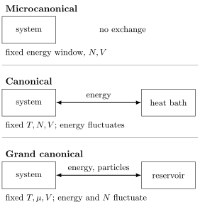
Permitted exchanges help identify an equilibrium ensemble. Isolation preserves the prepared energy distribution; equal microcanonical weights require the additional statistical assignment described below.

The three density operators

Let $\mathcal H_N$ be the correctly symmetrized fixed-number Hilbert space. The microcanonical state is uniform on a chosen energy shell:

$$\rho_{\mathrm{mc}}=\frac{\Pi_{E,\Delta E}}{W},\qquad \Pi_{E,\Delta E}=\mathbf1_{[E-\Delta E/2,E+\Delta E/2]}(H_N), \qquad W=\operatorname{Tr}\Pi_{E,\Delta E}.$$

The definition requires $0<W<\infty$. It maximizes entropy among states supported in that shell. A finite-dimensional or suitably confined system has discrete levels, so the window must be stated: selecting one nondegenerate level gives a pure state, whereas a many-level window gives a mixture. The shell entropy is $S=k_{\mathrm B}\ln W$; a smooth thermodynamic entropy defines $1/T=(\partial S/\partial E)_{N,V}$.

The canonical state weights energies at fixed particle number:

$$\rho_{\mathrm c}=\frac{e^{-\beta H_N}}{Z_N},\qquad Z_N=\operatorname{Tr}_{\mathcal H_N}e^{-\beta H_N}.$$

Its normalization gives the Helmholtz free energy $F=-k_{\mathrm B}T\ln Z_N$. A large bath supplies the factor $e^{-\beta E_n}$ because its number of compatible states decreases as energy is transferred to the subsystem. The reservoir derivation and its finite-bath correction are developed on the canonical page.

The grand-canonical state includes different number sectors:

$$\rho_{\mathrm{gc}}=\frac{e^{-\beta(H-\mu N)}}{\Xi},\qquad \Xi=\operatorname{Tr}_{\mathcal F}e^{-\beta(H-\mu N)} =\sum_N e^{\beta\mu N}Z_N.$$

Here $\mathcal F=\bigoplus_N\mathcal H_N$ is Fock space. Both partition functions must be finite. The grand potential is $\Omega_{\mathrm G}=-k_{\mathrm B}T\ln\Xi$. The operator $H-\mu N$ determines equilibrium weights; $H$ generates laboratory real-time evolution, unless a different frame is explicitly chosen.

The trace domain is essential. A trace over one fixed-$N$ sector does not acquire number fluctuations merely by inserting $-\mu N$: that term is constant in the sector and cancels from the normalized state.

What the ensemble predicts

The ensemble supplies the state in the usual quantum measurement rules:

$$\langle A\rangle=\operatorname{Tr}(\rho A),\qquad \Pr(a)=\operatorname{Tr}(\rho P_a).$$

Here $P_a$ is the projector for measurement outcome $a$. Thermal mixing and measurement uncertainty can both contribute. An energy eigenstate, for example, need not have a definite transverse spin.

For a temperature-independent Hamiltonian, the canonical energy variance is

$$\operatorname{Var}(H)=k_{\mathrm B}T^2 C_{V,N}.$$

This is an ensemble fluctuation, not uncertainty in the bath’s control setting. For a regular system with $C_{V,N}\propto V$, the fluctuation of energy density scales as $V^{-1/2}$. This statement is independent of the arbitrary zero of energy. It helps explain ensemble equivalence for local observables, but does not erase an exact global constraint or make all three density operators identical. Phase coexistence and nonadditive interactions need separate analysis.

Choosing the system boundary

A fixed-number atomic cloud and one small region of that cloud need not use the same ensemble. The whole cloud lies in $\mathcal H_{N_{\mathrm{tot}}}$; particles can still cross the smaller region’s boundary. If the rest acts as an equilibrium reservoir, that region may be approximately grand canonical.

A quantum dot weakly coupled to equilibrium leads at a common $T,\mu$ offers another grand-canonical example. Under a voltage bias the leads have different chemical potentials, so one global equilibrium state with a single $\mu$ generally fails.

For a spin with $H=-h\sigma_z$ in thermal equilibrium,

$$\rho=\frac{e^{\beta h\sigma_z}}{2\cosh(\beta h)}.$$

The two energies fluctuate even though the number of spins is fixed. A discrete spectrum therefore does not by itself select the microcanonical ensemble.

Equilibrium and dynamics answer different questions

Isolation preserves the initial energy probabilities. It does not make them equal, and unitary evolution preserves the entropy of the full density operator. A pure state after a quench remains pure even when local observables relax to thermal values. Such agreement requires a thermalization analysis.

Maximum entropy provides another derivation of the ensemble states from support or mean-value constraints; it is an inference principle, not a proof of relaxation. Additional conserved quantities may require a generalized Gibbs state. Strong subsystem–bath coupling can require a Hamiltonian of mean force.

Finally, the von Neumann entropy of a thermal mixed state is not generally an entanglement measure. For the relation between thermodynamic, reduced-state, and information entropies, see Entropy.

Exercises

Classify four preparations

Identify the most appropriate equilibrium description, or explain why none is exact:

1. a sealed many-body system with sharply specified total energy and particle number;
2. a fixed-number spin sample weakly coupled to a thermostat;
3. a quantum dot weakly coupled to one equilibrium particle reservoir;
4. an isolated pure state immediately after a sudden quench.

Solution

1. The microcanonical ensemble is the maximum-entropy assignment when only that shell and particle number are specified. Isolation alone does not turn a known pure preparation into a uniform mixture.
2. The canonical ensemble is appropriate: energy can be exchanged, while particle number is fixed.
3. The grand-canonical ensemble is the equilibrium reference: both energy and particle number can be exchanged.
4. The exact state is the unitarily evolving pure state, not an equilibrium ensemble. At late times, selected observables may agree with an equilibrium or generalized ensemble, but that requires a thermalization analysis.

Trace-space diagnostic

A number-conserving Hamiltonian has fixed-sector partition functions

$$Z_N = \operatorname{Tr}_{\mathcal H_N} e^{-\beta H_N}.$$

Show how the grand partition function is assembled from these sectors and identify the variable conjugate to $N$.

Solution

Fock space is the direct sum

$$\mathcal F = \bigoplus_{N=0}^{\infty} \mathcal H_N.$$

Therefore

$$\begin{aligned} \Xi &= \operatorname{Tr}_{\mathcal F} e^{-\beta(H-\mu N)} \\ &= \sum_{N=0}^{\infty} e^{\beta\mu N} \operatorname{Tr}_{\mathcal H_N} e^{-\beta H_N} \\ &= \sum_{N=0}^{\infty} z^N Z_N, \end{aligned}$$

where

$$z=e^{\beta\mu}.$$

The chemical potential $\mu$ is conjugate to particle number; equivalently, fugacity $z$ counts number sectors in the generating function.

A local grand-canonical state from a fixed total number

Let a total system $A\cup B$ have exactly $N_{\mathrm{tot}}$ particles. Explain how subsystem $A$ can nevertheless be approximately grand canonical.

Solution

Although

$$N_A+N_B = N_{\mathrm{tot}}$$

is fixed, the subsystem number $N_A$ can fluctuate because particles move between $A$ and $B$. If $B$ is much larger and remains near equilibrium, its entropy expansion for a transfer of energy and particles supplies the weight

$$p_{n,N_A} \propto \exp\!\left[ -\beta(E_{n,N_A}-\mu N_A) \right].$$

Thus the reduced equilibrium state of $A$ can be approximately grand canonical. Exact total-number conservation is fully compatible with local number fluctuations.

Ensemble and measurement uncertainty

Suppose a canonical state is diagonal in the energy basis:

$$\rho = \sum_n p_n|E_n\rangle\langle E_n|.$$

For an observable $A$ that does not commute with $H$, write the probability of outcome $a$ and explain the two sources of uncertainty.

Solution

If $P_a$ is the projector for outcome $a$, then

$$\Pr(a) = \operatorname{Tr}(\rho P_a) = \sum_n p_n \langle E_n|P_a|E_n\rangle.$$

The weights $p_n$ express the thermal mixture over energy states. For each energy state, the factor

$$\langle E_n|P_a|E_n\rangle$$

is the Born probability for the measurement of $A$. When $[A,H]\neq0$, an energy eigenstate need not give a definite value of $A$. Statistical uncertainty in the state and quantum measurement uncertainty can therefore appear in the same prediction.

References

• H. B. Callen, Thermodynamics and an Introduction to Thermostatistics, 2nd ed., Wiley (1985), chapters 1–7.
• K. Huang, Statistical Mechanics, 2nd ed., Wiley (1987), chapters 6–9.
• E. T. Jaynes, “Information Theory and Statistical Mechanics”, Physical Review 106, 620–630 (1957).
• M. Kardar, Statistical Physics of Particles, Cambridge University Press (2007), chapters 1–4.
• L. D. Landau and E. M. Lifshitz, Statistical Physics, Part 1, 3rd ed., Butterworth–Heinemann (1980), sections 1–35.
• R. K. Pathria and P. D. Beale, Statistical Mechanics, 4th ed., Elsevier (2021), especially the ensemble formulation and quantum-statistics chapters.
• D. Ruelle, Statistical Mechanics: Rigorous Results, W. A. Benjamin (1969), chapters 1–3.
• H. Tasaki, Physics and Mathematics of Quantum Many-Body Systems, Springer (2020), introductory discussion of many-body systems and thermodynamic limits.