Floquet Quantum Matter

Floquet quantum matter is matter whose useful dynamical structure is created or reorganized by a drive that repeats over many controlled cycles. The repeated drive can dress bands, renormalize tunneling and exchange, synthesize gauge fields, generate topology tied to an entire cycle, or stabilize long-lived subharmonic response. None of those outcomes follows merely from applying a periodic field. The drive must remain coherent long enough, the target structure must be resolved against broadening and heating, and the measured state must actually occupy the relevant Floquet modes.

The central experimental distinction is between the driven spectrum and the state occupying it. A resolved gap can change the available modes without preparing the distribution needed for the desired transport. Floquet Systems Preview explains heating, prethermal behavior and full-cycle topology; here we connect those results to drive calibration, spectroscopy, micromotion and material response.

Required background. Floquet Systems Preview supplies the many-body heating, resonance and prethermal limits of periodic driving. Floquet Theorem in Quantum Mechanics supplies the one-period propagator, quasienergies and micromotion. Chern Numbers in Band Theory supplies the Bloch-band invariant and the gap and filling assumptions needed when comparing band topology with measured transport.

Periodic driving over a finite time

An ideal Floquet Hamiltonian obeys strict periodicity. A laboratory drive also has an envelope, loading ramp, phase noise, spatial profile, and finite duration:

$$\begin{gathered} H(t+T)=H(t), \qquad \Omega=\frac{2\pi}{T}, \\ N_{\mathrm{cyc}} = \frac{\tau_{\mathrm{pulse}}}{T}. \end{gathered}$$

Here $\tau_{\mathrm{pulse}}$ is the interval over which the drive amplitude is approximately controlled. A quasienergy description is useful only if the system experiences enough phase-coherent cycles for the relevant observable. A ten-cycle pulse can reveal photon-dressed replicas without establishing a long-lived many-body phase.

The carrier frequency alone is insufficient: loading, envelope, polarization, phase noise and spatial inhomogeneity all affect the prepared state. Readout at a fixed phase of each cycle samples stroboscopic dynamics; readout between these times also sees micromotion, the motion within a period.

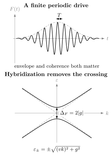
A finite coherent drive can hybridize quasienergy branches. The lower panel shows the eigenvalues $\varepsilon_\pm(k)=\pm\sqrt{(vk)^2+g^2}$ of a local two-level crossing model, where $vk$ is the uncoupled detuning and $g$ the coupling; the gap is $\Delta_F=2|g|$. Dashed lines are uncoupled branches. The upper waveform is illustrative, and the crossing model does not determine the occupations or topology of a whole band.

Calibrating the drive

For a charged Bloch system coupled through a vector potential, a common starting point is

$$H(\mathbf k,t) = H_0\!\left( \mathbf k-\frac{q}{\hbar}\mathbf A(t) \right).$$

If an approximately monochromatic electric field has amplitude $E_0$, then $A_0\sim E_0/\Omega$. A natural bond-scale drive strength is

$$\kappa = \frac{\lvert q\rvert aE_0}{\hbar\Omega},$$

where $a$ is the relevant hopping distance. Reporting only intensity hides the frequency dependence of $\kappa$. It also hides local-field corrections, screening, and polarization relative to crystal axes.

Optical-lattice shaking is often calibrated by displacement or inertial force rather than electric field. Digital spin and qubit experiments instead need pulse angles, gate order, coherent over-rotation, and idle evolution. These controls are not interchangeable, even when their leading effective Hamiltonians look alike.

The drive frequency must be compared with several scales:

• target bandwidths, gaps, interactions, and exchange energies;
• unwanted interband gaps and higher orbital levels;
• linewidths and dephasing rates;
• bath and phonon frequencies;
• the inverse ramp time and pulse bandwidth.

“High frequency” means high relative to the local processes retained in a declared model. It need not be high relative to every microscopic transition. Near-resonant engineering deliberately violates an off-resonant condition and therefore requires explicit leakage and occupation measurements.

Quasienergy in spectroscopy

Floquet quasienergy is defined modulo the drive quantum. In an extended-zone picture, a dressed band appears as replicas

$$\varepsilon_{\alpha m}(\mathbf k) = \varepsilon_\alpha(\mathbf k) +m\hbar\Omega, \qquad m\in\mathbb Z.$$

These shifted labels describe the same Floquet solution when accompanied by the matching change of periodic mode. They are not extra independently occupied bands. Quasienergy lives on a circle, so there is no globally preferred lowest quasienergy analogous to a static ground-state energy. Loading and scattering determine occupations.

Where distinct branches hybridize, a drive-induced avoided crossing can open. Resolving its gap requires enough coherent drive duration and sufficient probe energy resolution. The finite drive envelope, probe envelope, intrinsic linewidth and spectrometer response are separate effects.

For a transform-limited Gaussian probe amplitude

$$s(t)=e^{-t^2/(4\sigma_t^2)}, \qquad |\widetilde s(\omega)|^2\propto e^{-2\sigma_t^2\omega^2},$$

the probe intensity has temporal standard deviation $\sigma_t$ and energy standard deviation $\hbar/(2\sigma_t)$. In terms of intensity full widths at half maximum,

$$\delta E_{\mathrm{probe}}\,\tau_{\mathrm{probe}}=4\ln2\,\hbar.$$

Thus using a long drive does not remove broadening from a short probe. Gaussian contributions combine in quadrature, Lorentzian widths add under convolution, and mixed line shapes require an appropriate model. A gap comparable to the total width needs a line-shape fit and adequate signal-to-noise; a simple inverse-duration estimate is not a universal resolution threshold.

Time-resolved photoemission

Time- and angle-resolved photoemission does not directly photograph a quasienergy eigenvalue. Use the fermionic lesser convention

$$G^<_{\mathbf k}(t,t') = i\left\langle c^\dagger_{\mathbf k}(t')c_{\mathbf k}(t) \right\rangle.$$

For a real probe envelope $s$, angular frequency $\omega$ and delay $t_d$, with constant photoemission matrix elements suppressed, the intensity is schematically

$$I(\mathbf k,\omega;t_d) \propto -i \int dt\,dt'\, s(t-t_d)s(t'-t_d) \times e^{i\omega(t-t')} G^<_{\mathbf k}(t,t').$$

The factor $-i$ converts the lesser Green function to the occupied correlation entering a real, nonnegative intensity. For a complex probe envelope, replace the product by $s(t-t_d)s^*(t'-t_d)$. Pump–Probe Spectroscopy explains the measurement model and its gauge and resolution qualifications; Freericks, Krishnamurthy, and Pruschke derive the two-time expression.

The pulse envelope $s$, photoemission matrix elements, occupations, and final-state propagation all matter. A free photoelectron can itself be dressed by the pump, producing Volkov sidebands that resemble initial-state Floquet replicas. Floquet and Volkov pathways can also interfere.

Polarization, incidence angle, emission momentum and probe photon energy change the final-state coupling. Compare their joint dependence with calculations containing both pathways and their interference, and look for coherent avoided crossings when resolution permits. Mahmood et al. (2016) demonstrate why such controls matter. A sideband alone establishes neither a topological state nor quantized transport.

Cold-atom and synthetic platforms

Ultracold atoms do not provide electronic photoemission, but band mapping, state tomography, center-of-mass drift, circular dichroism, and quench dynamics can reconstruct quasienergy gaps and Berry-curvature information. The absence of a filled electronic Fermi sea is an advantage for state preparation but makes the measured response preparation dependent.

Photonic and acoustic platforms can image propagation and edge transport with exceptional spatial resolution. In many such systems a propagation coordinate plays the role of time. This faithfully tests a wave equation and its unitary topology, but it does not reproduce fermionic occupations, quantum thermalization, or energy absorption by an isolated many-body state.

Testing an effective Hamiltonian

An exact one-cycle matrix logarithm need not be a useful local effective Hamiltonian. Its validity depends on the stroboscopic phase, branch choice, ramp, state, observable, and time window.

For a chosen reference phase, write the periodic decomposition as $U(t,0)=P(t)e^{-iH_Ft/\hbar}$ with $P(0)=I$. The same approximation must predict both $H_F$ and the micromotion $P(t)$. A measured operator becomes

$$O_{\mathrm{eff}}(t)=P^\dagger(t)O P(t)$$

in that frame. Omitting this transformation can make a good effective Hamiltonian appear to fail between periods (Goldman and Dalibard, 2014; Bukov et al., 2015).

Fit a shared parameter set to selected data, then predict different observables and phases within a cycle. Compare with exact finite-drive evolution where possible, vary frequency and amplitude, and measure population outside the retained bands. Correlated errors require their covariance in any joint residual; matching one gap or stroboscopic population does not test currents, occupations and micromotion simultaneously.

Near a multiphoton resonance, denominators in an off-resonant expansion become small. The resonant states must then enter the explicit model. A resonant rotating-frame model may then be controlled even though the original off-resonant expansion is not.

What different platforms measure

Platform	Useful measurement and main limitation
Electronic solids	Spectra and ultrafast currents; coherence, occupation, phonons and penetration depth matter.
Optical lattices	Band mapping, geometric drift and heating; higher bands, traps and loading constrain interpretation.
Trapped ions and qubits	Local dynamics and subharmonic response; finite size, control errors and decoherence limit the window.
Photonic or acoustic lattices	Field reconstruction and edge propagation; wave dynamics does not reproduce fermionic occupations or thermalization.

The right conclusion is platform specific. A photonic edge mode can establish anomalous unitary topology without answering a heating question. A cold-atom heating curve can test prethermal scaling without demonstrating an electronic material. A solid-state Hall pulse can reveal a helicity-dependent transverse response while still requiring a model of carriers, contacts, and dissipation.

Band topology, cycle topology and transport

Periodic driving supports two distinct topological strategies:

1. engineer a static-looking effective band Hamiltonian with familiar Chern or symmetry invariants;
2. realize topology of the full evolution over a cycle, including anomalous edge modes not determined by Floquet-band Chern numbers alone.

Chern Numbers in Band Theory explains band invariants. For a driven system, a gap invariant can depend on the entire evolution, and chiral edge modes can occur even when every Floquet band has zero Chern number (Rudner et al., 2013). Bulk–Boundary Correspondence connects a specified gap and interface to boundary modes.

Measurement	What it determines and what remains separate
Replicas	Periodic dressing; final-state effects may contribute.
Avoided crossing	Coherent hybridization; a local gap does not fix a global invariant.
Berry-curvature-sensitive motion	Band geometry for the prepared distribution; occupations affect the response.
Transverse current	Transport under the stated contacts and drive; separate geometric and carrier-distribution contributions.
Gap-resolved edge propagation	Boundary behavior; identify the appropriate band or full-cycle invariant.

Even for noninteracting Floquet bands, transport depends on occupations. In a slow-probe band description with negligible interband coherence, an intrinsic cycle-averaged Hall contribution in two dimensions has the form (Dehghani, Oka and Mitra, 2015)

$$\sigma_{xy}^{\mathrm{band}} = -\frac{q^2}{\hbar} \sum_\alpha \int_{\mathrm{BZ}} \frac{d^2k}{(2\pi)^2} f_\alpha(\mathbf k) \Omega_\alpha^F(\mathbf k).$$

Here $f_\alpha$ is the occupation of a distinct Floquet mode and $\Omega_\alpha^F$ is its time-averaged Berry curvature. For a periodic Bloch mode $|u_{\alpha\mathbf k}(t)\rangle$, use

$$\mathbf A_\alpha^F=\frac{i}{T}\int_0^Tdt\, \langle u_{\alpha\mathbf k}(t)|\nabla_{\mathbf k}u_{\alpha\mathbf k}(t)\rangle, \qquad \Omega_\alpha^F=(\nabla_{\mathbf k}\times\mathbf A_\alpha^F)_z.$$

A generic partial or momentum-dependent occupation prevents quantization even when the band’s Chern number is nonzero. A fully occupied isolated band is a special limit. The measured conductivity may also contain distribution changes, interband processes and contact or bath effects; the full Floquet response requires the corresponding response calculation (Rudner and Lindner, 2020).

The shaken-lattice Haldane experiment combined gap closing with Berry-curvature-sensitive drift (Jotzu et al., 2014). Wintersperger et al. (2020) inferred anomalous Floquet invariants using gap measurements and local Hall deflections. Photonic lattices directly imaged robust edge propagation (Rechtsman et al., 2013). These are complementary tests, not interchangeable demonstrations of one universal phase.

Heating, dephasing and the observation window

A first estimate of the useful window takes the shortest relevant timescale:

$$\tau_{\mathrm{use}} = \min \left( \tau_\phi, \tau_{\mathrm{heat}}, \tau_{\mathrm{loss}}, \tau_{\mathrm{pulse}}, \tau_{\mathrm{drift}} \right).$$

For an engineered gap or coupling $\Delta_{\mathrm{eng}}$, define

$$Q_F = \frac{ \Delta_{\mathrm{eng}}\tau_{\mathrm{use}} }{\hbar}.$$

This counts characteristic phase-evolution times $\hbar/\Delta_{\mathrm{eng}}$, not full oscillations. A beat between two modes separated by $\Delta_{\mathrm{eng}}$ has period $2\pi\hbar/\Delta_{\mathrm{eng}}$, so it completes approximately $Q_F/(2\pi)$ cycles in the available window. Small $Q_F$ obstructs coherent gap dynamics; large $Q_F$ does not by itself prepare the desired state. Rates acting on the same observable can add, so the minimum-time estimate is only a first approximation.

In bounded, nearly isolated lattice models, generic periodic driving can lead toward sector-constrained infinite-temperature local behavior. At high local frequency, absorption can be exponentially slow and a prethermal effective Hamiltonian can govern a long interval. Prethermalization Preview explains the plateau and escape criteria. Rubio-Abadal et al. (2020) measured frequency-dependent suppression of heating in a Bose–Hubbard system.

Real materials exchange energy with phonons, substrates, leads and photons. A steady signal can reflect a balance between absorption and cooling rather than an isolated Floquet eigenstate. Atom loss can also carry away high-energy particles, so the temperature of those remaining need not measure total absorption (Reitter et al., 2017). Driven Many-Body Systems explains energy balance; Driven Open Systems develops periodic reduced-state dynamics.

Subharmonic response

A discrete time crystal responds with a robust integer multiple of the drive period. A subharmonic Fourier peak alone can also result from beating, control errors, aliasing or synchronization with an environment. The relevant tests include locking over a parameter interval, interactions, spatial correlations and lifetime scaling. Floquet Systems Preview explains localized and prethermal mechanisms. Floquet and Driven Systems research follows open questions about realistic stability and useful lifetimes.

Exercises

1. Can the pulse resolve the gap?

A drive with $\hbar\Omega=0.20\ \mathrm{eV}$ has a nearly flat $300\ \mathrm{fs}$ plateau. A transform-limited Gaussian probe has intensity FWHM $100\ \mathrm{fs}$. Suppose intrinsic and additional instrumental energy broadening are Gaussian with FWHM $12$ and $8\ \mathrm{meV}$. Estimate the number of drive cycles and total energy width for a proposed $20\ \mathrm{meV}$ gap. Use $\hbar=0.658\ \mathrm{eV\,fs}$.

Solution

The period and drive-cycle count are

$$T=\frac{2\pi\hbar}{\hbar\Omega}\simeq20.7\ \mathrm{fs}, \qquad N_{\mathrm{cyc}}\simeq14.5.$$

The Gaussian probe contributes

$$\delta E_{\mathrm{probe}}=\frac{4\ln2\,\hbar}{\tau_{\mathrm{probe}}} \simeq18.2\ \mathrm{meV}.$$

For the assumed Gaussian line shapes,

$$\delta E_{\mathrm{total}}\simeq\sqrt{12^2+8^2+18.24^2}\ \mathrm{meV} \simeq23.3\ \mathrm{meV}.$$

The proposed gap is smaller than this width, so the durations alone do not support a clearly resolved gap. Detailed spectral fitting may still constrain it, depending on signal-to-noise and matrix elements. The $300\ \mathrm{fs}$ drive duration cannot replace the $100\ \mathrm{fs}$ probe duration in this estimate; finite-envelope drift or additional decoherence can only worsen this simple stationary-plateau comparison.

2. Field amplitude versus Floquet coupling

Two experiments use the same electric-field amplitude $E_0$ and lattice spacing $a$, but experiment B uses half the angular frequency of experiment A. Compare their dimensionless Peierls strengths $\kappa$. Does this prove that B gives better off-resonant engineering?

Solution

Because

$$\kappa = \frac{\lvert q\rvert aE_0}{\hbar\Omega},$$

halving $\Omega$ doubles $\kappa$. This increases the momentum excursion and can strengthen dressing.

It does not establish better off-resonant engineering. The lower frequency may approach intraband, interband, phonon, or many-body resonances; it also narrows the separation between the drive quantum and local energy scales. Leakage and absorption can therefore increase even while $\kappa$ becomes larger.

3. Test an effective Hamiltonian without refitting

An effective model is fitted to stroboscopic density data at one frequency. Propose a held-out test that addresses both micromotion and parameter transfer.

Solution

First freeze all fitted parameters. At the original drive setting, measure a current or correlation function at several phases $\tau$ within the cycle and compare it with the model using the properly dressed observable. This tests micromotion.

Then change the frequency while preserving the calibrated dimensionless drive strength and predict the new data without refitting microscopic couplings. A successful model should reproduce several observables and their phase dependence over a declared time window. Failure localized near a resonance indicates that omitted states or resonant processes must enter the model.

4. Compute the usable Floquet window

A driven device has $T=25\ \mathrm{fs}$, $\tau_\phi=180\ \mathrm{fs}$, $\tau_{\mathrm{heat}}=2.5\ \mathrm{ps}$, $\tau_{\mathrm{loss}}=8\ \mathrm{ps}$, and $\tau_{\mathrm{pulse}}=400\ \mathrm{fs}$. Its engineered gap is $15\ \mathrm{meV}$. Estimate $N_{\mathrm{use}}$ and $Q_F$.

Solution

Dephasing is the shortest timescale, so

$$\tau_{\mathrm{use}} = 180\ \mathrm{fs}, \qquad N_{\mathrm{use}} = \frac{180}{25} = 7.2.$$

Using $\hbar=658\ \mathrm{meV\,fs}$,

$$Q_F = \frac{ (15\ \mathrm{meV})(180\ \mathrm{fs}) }{ 658\ \mathrm{meV\,fs} } \approx 4.1.$$

There are about seven drive cycles but only $Q_F/(2\pi)\simeq0.65$ full gap-beat oscillations. These count different motions. The estimate permits some coherent dressing, but does not establish resolved gap oscillations or precise transport. Improving only the heating time leaves dephasing as the limiting process.

References

• M. Bukov, L. D’Alessio, and A. Polkovnikov, “Universal High-Frequency Behavior of Periodically Driven Systems: From Dynamical Stabilization to Floquet Engineering,” Advances in Physics 64, 139–226 (2015), doi:10.1080/00018732.2015.1055918. Reviews gauge, micromotion, and high-frequency engineering.
• H. Dehghani, T. Oka, and A. Mitra, “Out-of-Equilibrium Electrons and the Hall Conductance of a Floquet Topological Insulator,” Physical Review B 91, 155422 (2015), doi:10.1103/PhysRevB.91.155422. Relates cycle-averaged Berry curvature and occupations to the dc Hall response.
• A. Eckardt, “Colloquium: Atomic Quantum Gases in Periodically Driven Optical Lattices,” Reviews of Modern Physics 89, 011004 (2017), doi:10.1103/RevModPhys.89.011004. Reviews optical-lattice implementations and limitations.
• J. K. Freericks, H. R. Krishnamurthy, and Th. Pruschke, “Theoretical Description of Time-Resolved Photoemission Spectroscopy: Application to Pump–Probe Experiments,” Physical Review Letters 102, 136401 (2009), doi:10.1103/PhysRevLett.102.136401; erratum 119, 189903 (2017), doi:10.1103/PhysRevLett.119.189903. Derives the probe-windowed lesser-Green expression and its normalization.
• N. Goldman and J. Dalibard, “Periodically Driven Quantum Systems: Effective Hamiltonians and Engineered Gauge Fields,” Physical Review X 4, 031027 (2014), doi:10.1103/PhysRevX.4.031027. Develops effective Hamiltonians and micromotion for engineered gauge fields.
• G. Jotzu et al., “Experimental Realization of the Topological Haldane Model with Ultracold Fermions,” Nature 515, 237–240 (2014), doi:10.1038/nature13915. Realizes an effective driven Haldane band in an optical lattice.
• F. Mahmood et al., “Selective Scattering between Floquet–Bloch and Volkov States in a Topological Insulator,” Nature Physics 12, 306–310 (2016), doi:10.1038/nphys3609. Demonstrates the importance of final-state dressing in photoemission.
• M. C. Rechtsman et al., “Photonic Floquet Topological Insulators,” Nature 496, 196–200 (2013), doi:10.1038/nature12066. Directly images robust photonic edge propagation.
• M. Reitter et al., “Interaction Dependent Heating and Atom Loss in a Periodically Driven Optical Lattice,” Physical Review Letters 119, 200402 (2017), doi:10.1103/PhysRevLett.119.200402. Resolves interaction, interband, heating, and loss channels.
• A. Rubio-Abadal et al., “Floquet Prethermalization in a Bose–Hubbard System,” Physical Review X 10, 021044 (2020), doi:10.1103/PhysRevX.10.021044. Measures frequency-dependent suppression of heating.
• M. S. Rudner and N. H. Lindner, “Band Structure Engineering and Non-Equilibrium Dynamics in Floquet Topological Insulators,” Nature Reviews Physics 2, 229–244 (2020), doi:10.1038/s42254-020-0170-z. Separates band topology, occupations, heating, and observable response.
• M. S. Rudner, N. H. Lindner, E. Berg, and M. Levin, “Anomalous Edge States and the Bulk–Edge Correspondence for Periodically Driven Two-Dimensional Systems,” Physical Review X 3, 031005 (2013), doi:10.1103/PhysRevX.3.031005. Establishes full-cycle anomalous Floquet topology.
• K. Wintersperger et al., “Realization of an Anomalous Floquet Topological System with Ultracold Atoms,” Nature Physics 16, 1058–1063 (2020), doi:10.1038/s41567-020-0949-y. Combines gap and local-Hall measurements to infer anomalous invariants.

Further Reading

• D. V. Else, C. Monroe, C. Nayak, and N. Y. Yao, “Discrete Time Crystals,” Annual Review of Condensed Matter Physics 11, 467–499 (2020), doi:10.1146/annurev-conmatphys-031119-050658. Reviews definitions, stabilization mechanisms, and experimental diagnostics.
• M. A. Sentef et al., “Theory of Floquet Band Formation and Local Pseudospin Textures in Pump–Probe Photoemission of Graphene,” Nature Communications 6, 7047 (2015), doi:10.1038/ncomms8047. Connects driven pseudospin dynamics to time-resolved spectra.