Driven-Dissipative Matter

Driven-dissipative matter is many-body matter whose persistent state is selected by sustained input together with loss, dephasing, or particle exchange. It is not a closed material weakly perturbed by a probe. Turning off the pump generally removes the state itself, while turning off the loss generally changes or destabilizes it. The generator, reservoirs, boundaries, and measurement ports are therefore part of the physical specification.

The central questions are what is supplied, where it goes, and which measurements distinguish coherent order from a bright stationary output. We develop a simple pumped mode and a polariton reservoir model, then connect them to coherence and collective transitions. Driven Open Systems explains the master-equation framework; Open Quantum Materials treats non-Hermitian spectra and exceptional points.

Required background. Driven Many-Body Systems supplies external forcing, energy balance and heating regimes. Driven Open Systems supplies the combined treatment of time-dependent control and environmental exchange. Steady States and Relaxation supplies generator fixed points, relaxation modes and uniqueness conditions. Bose–Einstein Condensation supplies the macroscopic one-body-density-matrix eigenvalue criterion, which can be distinguished from equilibrium and transport claims.

Steady matter far from equilibrium

The Hamiltonian alone does not select a driven state. Injection spectra, loss channels, bath temperatures and boundaries also matter: two devices with the same rotating-frame Hamiltonian can settle into different states. Specify whether the measured quantity is stationary in the laboratory frame, stationary in a rotating frame or periodic with the drive.

A stationary density operator does not imply equilibrium. A nonequilibrium steady state can carry a constant particle, photon, spin, or energy current. Its entropy can remain constant while entropy is continually exported. A time-independent measured intensity can likewise conceal switching between metastable states, phase diffusion, or unresolved periodic motion.

Pumping and loss

Pumping can be coherent or incoherent. A coherent drive fixes a phase reference and directly contributes a term such as $F a^\dagger+F^*a$ to a rotating-frame Hamiltonian. An incoherent pump populates a reservoir or mode without fixing the condensate phase and is often represented by transition rates or jump operators. The distinction matters for symmetry: a coherent source can explicitly break a $U(1)$ phase symmetry that an incoherent pump leaves available for spontaneous ordering.

Radiative escape, nonradiative recombination, particle loss and pure dephasing are different channels. Pure dephasing can destroy coherence without removing particles; boundary leakage transports particles out of the chosen region. Keep these mechanisms separate when comparing detector counts with an internal occupation.

The number balance is

$$\frac{d}{dt} \langle N\rangle = R_{\mathrm{in}} - R_{\mathrm{out}} - R_{\mathrm{nr}} + J_{\partial}.$$

$J_{\partial}$ is positive when particles enter through a retained boundary. At a stationary operating point, the right-hand side vanishes. This expresses conservation at the chosen operating point; it does not fix coherence or an equilibrium distribution.

The energy balance counts distinct fluxes across the same boundary. For example, after steady-state averaging,

$$0=P_{\mathrm{abs}}-P_{\mathrm{rad}}-P_{\mathrm{heat,out}}-P_{\mathrm{matter,out}}.$$

Internal nonradiative recombination may first transfer energy to phonons and then to outgoing heat. Counting both steps as independent energy losses from the full device would double count the same energy. A finite internal energy or occupation can coexist with continuous absorption and outward flux.

A minimal birth–death mode

Consider a bosonic mode with incoherent single-particle pump coefficient $P$, population-loss rate $\kappa$, and a number-conserving Hamiltonian, such as $H=\hbar\omega a^\dagger a$. Thus $[H,n]=0$ for $n=a^\dagger a$; no coherent source is included in this minimal model:

$$\dot\rho = -\frac{i}{\hbar}[H,\rho] + P\mathcal D[a^\dagger]\rho + \kappa\mathcal D[a]\rho,$$

where

$$\mathcal D[L]\rho = L\rho L^\dagger - \frac{1}{2} \left\{ L^\dagger L,\rho \right\}.$$

For $n=a^\dagger a$,

$$\frac{d}{dt}\langle n\rangle = P\left( \langle n\rangle+1 \right) - \kappa\langle n\rangle.$$

If $P<\kappa$, the stationary occupation is

$$\langle n\rangle_{\mathrm{ss}} = \frac{P}{\kappa-P}.$$

The stationary number distribution is geometric,

$$p_n=(1-r)r^n,\qquad 0<r=P/\kappa<1, \qquad g^{(2)}(0)=2.$$

The pump includes bosonic stimulation through the factor $n+1$. Even a large mean occupation remains bunched in this model; it does not become a coherent laser field merely because pump nearly balances loss. At $P=\kappa$ no normalizable stationary distribution remains. Saturation, nonlinear loss, pump depletion or another mechanism is needed to stabilize a real device above this linear threshold. Number-conserving interactions alone do not fix this population runaway with the stated constant Markovian rates.

With a coherent source $Fa^\dagger+F^*a$, the number equation additionally contains $i\langle F^*a-Fa^\dagger\rangle/\hbar$ and does not close on the mean occupation. Pump coherence therefore changes both the symmetry and the equations.

Exciton–polaritons

Exciton–polaritons are hybrid light–matter quasiparticles formed when a confined photon mode and an exciton remain in the strong-coupling regime. For one in-plane momentum, a simple coupled-mode Hamiltonian is

$$H_{\mathrm{xc}} = \begin{pmatrix} E_C & g \\ g & E_X \end{pmatrix},$$

with eigenenergies

$$E_{\pm} = \frac{E_C+E_X}{2} \pm \frac{1}{2} \sqrt{ \left( E_C-E_X \right)^2 +4g^2 }.$$

The anticrossing and linewidths must demonstrate that the hybrid branches remain resolved in the regime being discussed. At high density, screening, phase-space filling, heating, or other nonlinearities can weaken strong coupling and permit an ordinary photon-lasing regime. Calling all coherent microcavity emission “polariton condensation” erases this distinction.

Polaritons combine a small photon-derived effective mass with exciton-derived interactions, but they also inherit radiative loss. A sustained population therefore requires pumping. Nonresonant pumping commonly creates an excitonic reservoir that relaxes into lower-polariton states; resonant pumping instead injects a selected polariton mode with a controlled phase and momentum. These protocols realize different symmetries and different fluctuation problems.

Open-dissipative Gross–Pitaevskii model

The mean-field reservoir model of Wouters and Carusotto (2007), in a form linear in reservoir gain, couples a complex polariton field $\psi(\mathbf r,t)$ to a reservoir density $n_R(\mathbf r,t)$:

$$\begin{aligned} i\hbar\partial_t\psi ={}& \left[ -\frac{\hbar^2\nabla^2}{2m} +V(\mathbf r) +g_C\lvert\psi\rvert^2 +g_R n_R \right]\psi + \frac{i\hbar}{2} \left( R n_R-\gamma_C \right)\psi, \\ \partial_t n_R ={}& P(\mathbf r,t) - \left( \gamma_R+R\lvert\psi\rvert^2 \right)n_R. \end{aligned}$$

Here $|\psi|^2$ and $n_R$ are densities. Accordingly $P$ is now a density injection rate, unlike the single-mode rate coefficient above; $R$ has units of inverse density per time. $m$ is the lower-polariton mass, $g_C$ is the condensate interaction, $g_R$ is the reservoir-induced shift, $R$ is the stimulated scattering coefficient, and $\gamma_C,\gamma_R$ are condensate and reservoir loss rates. The imaginary term is gain minus loss; it is not an imaginary conservative potential.

For a homogeneous time-independent pump, the zero-condensate solution has $n_R=P/\gamma_R$. Linear gain begins when

$$R n_R=\gamma_C,$$

so the mean-field threshold is

$$P_{\mathrm{th}} = \frac{\gamma_C\gamma_R}{R}.$$

Above threshold, a uniform solution with stationary densities clamps the reservoir and grows the condensate:

$$\begin{aligned} n_R^{\mathrm{ss}} &= \frac{\gamma_C}{R}, \\ \lvert\psi_{\mathrm{ss}}\rvert^2 &= \frac{ P-P_{\mathrm{th}} }{ \gamma_C }. \end{aligned}$$

The field itself generally rotates in phase. With uniform $V$,

$$\psi(t)=\sqrt{n_C}\,e^{-i\mu t/\hbar}, \qquad \mu=V+g_C n_C+g_R n_R^{\mathrm{ss}}.$$

Calling this stationary refers to its density or to the corresponding rotating frame. Gain balance does not establish stability against spatial perturbations; the coupled condensate and reservoir equations must be linearized around the solution. Eliminating the reservoir instantaneously also requires its relaxation rate $\gamma_R+Rn_C$ to exceed the frequencies being modeled. Near a slow mode that assumption should be checked again.

Finite spots introduce flow and boundary losses; spin, disorder, frequency-dependent gain and additional reservoirs change the dynamics. Fluctuations become particularly important near threshold and in low dimensions.

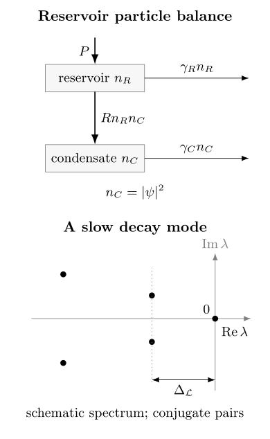
The reservoir transfers particles to the condensate at density rate $Rn_Rn_C$, with $n_C=|\psi|^2$; the same term enters their number equations with opposite signs. Below, a schematic Liouvillian spectrum illustrates the slowest decay rate. It is not a spectrum calculated from the reservoir model. A small finite gap and gap closure in a size limit are different statements.

What the mean-field model does not certify

A deterministic mean-field model can describe density profiles, blueshifts and instabilities without determining quantum noise or long-distance coherence. Fit parameters to one set of measurements and predict others, such as the reservoir shift, flow or relaxation spectrum. A fit to intensity alone cannot establish equilibrium, quantum fluctuations, superfluidity or a universality class (Carusotto and Ciuti, 2013).

Condensation, lasing and superfluidity

A threshold and a narrow line are shared by several coherent emitters. Stronger identification uses a bundle of observables.

Question	Useful measurement and main limitation
Are the modes polaritonic?	Resolve strong-coupling dispersion at the actual operating density.
Is occupation macroscopic?	Calibrate mode populations and the collection window.
Is phase coherence spontaneous?	Measure first-order coherence and exclude an imprinted pump phase.
What are the number fluctuations?	Measure intensity correlations with adequate timing and background correction.
Is there superfluid response?	Test drag, flow or circulation while controlling density, lifetime and defects.

For a stationary field with time-independent densities, first-order coherence can be written

$$g^{(1)}(\mathbf r,\mathbf r';\tau) = \frac{ \left\langle \psi^\dagger(\mathbf r,t) \psi(\mathbf r',t+\tau) \right\rangle }{ \sqrt{ n(\mathbf r)n(\mathbf r') } },$$

while intensity correlations use

$$g^{(2)}(0) = \frac{ \left\langle a^\dagger a^\dagger aa \right\rangle }{ \langle a^\dagger a\rangle^2 }.$$

Interferometry measures spatial or temporal coherence only after accounting for finite resolution, phase drift, and multimode emission. A value $g^{(2)}(0)\approx1$ is consistent with Poissonian number statistics but does not determine the full number distribution or prove a pure coherent state, a definite phase or a particular gain mechanism. Exercise 4 gives a counterexample.

Kasprzak and collaborators combined low-momentum occupation, temporal coherence, long-range spatial coherence, and polarization in their evidence for polariton condensation. Amo and collaborators tested fluid response by comparing defect scattering below and above the sound-speed scale. Those are different claims: condensation does not automatically imply superfluidity, and suppressed scattering should be checked against trivial changes in density, linewidth, or defect coupling.

Driven condensates can also have universal fluctuations with no equilibrium counterpart. In a suitable one-dimensional polariton lattice, Fontaine and collaborators measured spatiotemporal coherence scaling consistent with Kardar–Parisi–Zhang universality. Such a claim requires scaling functions or exponents over controlled windows, not merely a rough phase profile.

Measuring the emitted field

Polaritons, nonlinear optical resonators, circuit-QED arrays and atoms in optical cavities all connect collective dynamics to outgoing radiation. Their dominant complications differ: strong-coupling crossover in polaritons, technical noise in optical resonators, disorder and bandwidth in circuits, or reservoir elimination and atom-number drift in atom–cavity experiments. Artificial Lattices and Designer Matter compares these platforms.

The output is not a passive photograph of an isolated state. In a one-sided Markovian port (Gardiner and Collett, 1985),

$$a_{\mathrm{out}}(t) = a_{\mathrm{in}}(t) - \sqrt{\kappa_{\mathrm{ext}}}\,a(t),$$

with the stated minus-sign phase convention; $\kappa_{\mathrm{ext}}$ is the population decay rate into that port. The measured field contains interference between prompt input and cavity emission. Intracavity occupation cannot therefore be inferred from transmitted intensity without an input–output calibration.

Open-system phase transitions

For a time-independent Markovian model,

$$\dot\rho=\mathcal L\rho.$$

Let right eigenoperators obey

$$\mathcal L R_j = \lambda_j R_j, \qquad \lambda_0=0.$$

When the steady state is unique and the remaining modes decay, a common spectral gap is

$$\Delta_{\mathcal L} = -\max_{j\ne0} \operatorname{Re}\lambda_j.$$

The generic definitions and nonnormality cautions belong to Steady States and Relaxation. For material claims, the key point is operational: a small gap allows a long asymptotic relaxation time, but the initial state and measured observable must overlap the slow mode to reveal it. Nonnormal transients and multiple modes can complicate a fitted decay. One long time at one size does not establish gap closure.

Finite systems and singular limits

For a finite-dimensional generator that depends analytically on a parameter, an isolated simple stationary eigenvalue gives an analytic stationary state locally. A coalescence of nonzero decaying eigenvalues need not make that state singular. Sharp nonanalytic stationary behavior ordinarily requires loss of these conditions or a specified singular limit. That limit may be:

• the number of lattice sites $L\to\infty$;
• a large occupation or weak-noise limit;
• increasing atom number or cooperativity;
• a mode-volume scaling that keeps nonlinear energy extensive;
• a continuum or long-wavelength limit.

The scaling prescription is part of the phase definition. Increasing drive power alone is not automatically a thermodynamic limit, because it can also change heating, saturation, microscopic parameters, and the number of active modes.

Near a first-order dissipative transition, a finite system can show a bimodal field distribution and rare switching between dim and bright metastable states. The stationary mean then lies between two values that no single trajectory occupies for long. Histograms and dwell-time distributions are more informative than the mean (Casteels, Fazio and Ciuti, 2017; Minganti and collaborators, 2018).

Why hysteresis is not enough

Hysteresis can arise from metastable switching, a slow reservoir, detector filtering, thermal drift or a sweep faster than relaxation. Hold the control fixed within the loop and compare long time traces, distributions and relaxation rates. Then vary sweep and waiting times, detector bandwidth and a physically defined size parameter. The response must distinguish intrinsic switching from lag.

Rodriguez and collaborators measured sweep-time dependence of optical hysteresis in a semiconductor microcavity. Fitzpatrick and collaborators observed bistability and long switching times in a 72-site circuit-QED lattice. Fink and collaborators resolved bimodal phase-space distributions across photon-blockade breakdown. These experiments measure complementary aspects of switching and metastability; a hysteresis loop alone is insufficient to identify a phase transition.

A laser threshold, a dissipative phase transition, a dynamical instability, and an exceptional point are not synonyms. A laser threshold concerns gain, loss, and coherence onset. A dissipative transition concerns a singular change of the stationary state in a declared limit. An instability concerns linearized dynamics around a solution. An exceptional point concerns eigenvalue and eigenvector coalescence of a non-Hermitian operator; Open Quantum Materials explains the distinction.

Response, noise and effective temperature

A Lindblad equation gives a density-operator evolution for a specified Markovian model; a Schwinger–Keldysh theory can organize response, noise and collective fluctuations, including a field-theory description derived from that same model. They are compatible approaches at different levels. Colored noise and memory require their own treatment rather than an arbitrary time-local dissipator (Sieberer, Buchhold and Diehl, 2016).

For a stationary Hermitian fluctuation operator $\phi$ with zero mean, use the convention

$$\begin{aligned} G^R(t) &= -i\theta(t) \left\langle [\phi(t),\phi(0)] \right\rangle, \\ G^K(t) &= -i \left\langle \{\phi(t),\phi(0)\} \right\rangle. \end{aligned}$$

With the Fourier transform $G(\omega)=\int dt\,e^{i\omega t}G(t)$, thermal equilibrium relates the nonzero-frequency parts by the bosonic fluctuation–dissipation relation

$$G^K(\omega) = \coth\!\left( \frac{\hbar\omega}{2k_B T} \right) \left[ G^R(\omega)-G^A(\omega) \right].$$

A conserved fluctuation can retain a zero-frequency delta peak even after its mean is subtracted. This static weight must be supplied separately: the singular $\coth$ factor cannot recover it from a vanishing commutator. The equilibrium closure explains this qualification and the requirement that the thermal state and time evolution use the same generator.

A driven steady state generally has independent response and noise sectors. Fitting one low-frequency ratio by an effective temperature does not prove a global Gibbs state; the inferred temperature may depend on frequency, momentum, and observable. Schwinger–Keldysh Bridge develops the contour construction and consistency conditions.

Exercises

1. Linear pump threshold

For the birth–death mode with $[H,n]=0$, solve the mean occupation from initial value $n_0$. Derive the stationary distribution from adjacent probability fluxes and explain what changes at $P=\kappa$.

Solution

For $P\ne\kappa$,

$$\langle n(t)\rangle = \frac{P}{\kappa-P} + \left( n_0-\frac{P}{\kappa-P} \right) e^{-(\kappa-P)t}.$$

For $P<\kappa$, the mode relaxes to $P/(\kappa-P)$. At $P=\kappa$, the rate equation becomes $\dot n=P$, so occupation grows linearly. For $P>\kappa$, it grows exponentially. The latter regimes reveal the absence of saturation or nonlinear loss in the model; they do not predict an indefinitely growing real device.

At stationarity the adjacent fluxes balance:

$$P(n+1)p_n=\kappa(n+1)p_{n+1}.$$

Thus $p_{n+1}=rp_n$ with $r=P/\kappa$. Normalization gives $p_n=(1-r)r^n$ only for $r<1$. Summing its first two factorial moments yields $\langle n\rangle=r/(1-r)$ and $\langle n(n-1)\rangle=2\langle n\rangle^2$, hence $g^{(2)}(0)=2$ for nonzero pumping.

2. Reservoir threshold and clamping

For the homogeneous open-dissipative Gross–Pitaevskii equations, derive $P_{\mathrm{th}}$, $n_R^{\mathrm{ss}}$, and $\lvert\psi_{\mathrm{ss}}\rvert^2$ above threshold.

Solution

Below threshold, $\psi=0$ and stationarity gives $n_R=P/\gamma_R$. The field becomes marginal when $Rn_R=\gamma_C$, hence

$$P_{\mathrm{th}} = \frac{\gamma_C\gamma_R}{R}.$$

For a nonzero stationary condensate, gain balance fixes $n_R^{\mathrm{ss}}=\gamma_C/R$. The reservoir equation then gives

$$P = \left( \gamma_R+R\lvert\psi_{\mathrm{ss}}\rvert^2 \right) \frac{\gamma_C}{R},$$

and therefore

$$\lvert\psi_{\mathrm{ss}}\rvert^2 = \frac{P-P_{\mathrm{th}}}{\gamma_C}.$$

The clamping is a property of this homogeneous mean-field reduction, not a universal microscopic law.

3. Dynamic hysteresis

An optical cavity shows a wide hysteresis loop for a fast frequency sweep and a much narrower loop when the sweep is slowed. Give two interpretations and one measurement that helps distinguish them.

Solution

The loop can reflect metastable switching near a first-order dissipative transition, or it can be a purely dynamic lag caused by a reservoir, thermal drift, or detector response. Holding the control parameter fixed inside the loop and recording long time traces tests for stationary bimodality and stochastic switching. Varying the hold time, sweep time, and detector bandwidth helps separate intrinsic switching from instrumental lag.

4. Poisson statistics without a definite phase

Average a coherent state of amplitude $\alpha=\sqrt{\bar n}e^{i\theta}$ uniformly over its phase. Find the density matrix, $\langle a\rangle$ and $g^{(2)}(0)$ for $\bar n>0$. Does $g^{(2)}(0)=1$ prove a pure coherent state?

Solution

Phase averaging removes the off-diagonal number-state matrix elements:

$$\rho=\sum_{n=0}^\infty e^{-\bar n}\frac{\bar n^n}{n!}|n\rangle\langle n|.$$

The mean field vanishes, $\langle a\rangle=0$, while the Poisson distribution has $\langle n(n-1)\rangle=\bar n^2$ and therefore $g^{(2)}(0)=1$. The state is mixed and has no preferred phase. Equal-time number statistics cannot distinguish it from a coherent state of fixed phase; a phase reference and appropriate interference measurements probe different information. A vanishing ensemble mean field also does not, by itself, rule out coherence in individual realizations.

Current questions about preparation, scaling and reservoir robustness are discussed in Dissipation Engineering research. The models here specify finite systems and controlled approximations; their stationary solutions do not alone establish a thermodynamic phase.

References

• A. Amo, J. Lefrère, S. Pigeon, et al., “Superfluidity of polaritons in semiconductor microcavities,” Nature Physics 5, 805–810 (2009).
• I. Carusotto and C. Ciuti, “Quantum fluids of light,” Reviews of Modern Physics 85, 299–366 (2013).
• W. Casteels, R. Fazio, and C. Ciuti, “Critical dynamical properties of a first-order dissipative phase transition,” Physical Review A 95, 012128 (2017).
• J. M. Fink, A. Dombi, A. Vukics, A. Wallraff, and P. Domokos, “Observation of the photon-blockade breakdown phase transition,” Physical Review X 7, 011012 (2017).
• M. Fitzpatrick, N. M. Sundaresan, A. C. Y. Li, J. Koch, and A. A. Houck, “Observation of a dissipative phase transition in a one-dimensional circuit QED lattice,” Physical Review X 7, 011016 (2017).
• Q. Fontaine, D. Squizzato, F. Baboux, et al., “Kardar–Parisi–Zhang universality in a one-dimensional polariton condensate,” Nature 608, 687–691 (2022).
• C. W. Gardiner and M. J. Collett, “Input and output in damped quantum systems: Quantum stochastic differential equations and the master equation,” Physical Review A 31, 3761–3774 (1985).
• J. Kasprzak, M. Richard, S. Kundermann, et al., “Bose–Einstein condensation of exciton polaritons,” Nature 443, 409–414 (2006).
• F. Minganti, A. Biella, N. Bartolo, and C. Ciuti, “Spectral theory of Liouvillians for dissipative phase transitions,” Physical Review A 98, 042118 (2018).
• S. R. K. Rodriguez, W. Casteels, F. Storme, et al., “Probing a dissipative phase transition via dynamical optical hysteresis,” Physical Review Letters 118, 247402 (2017).
• L. M. Sieberer, M. Buchhold, and S. Diehl, “Keldysh field theory for driven open quantum systems,” Reports on Progress in Physics 79, 096001 (2016).
• M. Wouters and I. Carusotto, “Excitations in a nonequilibrium Bose–Einstein condensate of exciton polaritons,” Physical Review Letters 99, 140402 (2007).