Random Matrix Theory in Quantum Matter

Random matrix theory studies probability distributions on matrices and the universal spectral fluctuations that survive after system-specific scales have been removed. In quantum matter, its main role is not to claim that a microscopic Hamiltonian has independently random entries. It is to provide symmetry-controlled benchmarks for energy levels, quasienergies, scattering matrices, and certain eigenvector observables.

The examples below concern Hermitian spectra and unitary evolution, with one irreducible symmetry sector analyzed at a time. First identify which levels can mix, then remove the smooth variation in their density, and finally compare fluctuations. This order matters: pooling independent sectors or comparing raw gaps can hide level repulsion. Non-Hermitian spectra require a different framework.

Required background. Spectral Theorem, Practical Version supplies Hermitian spectral decomposition and projectors. Time Reversal supplies antiunitary symmetry and the distinction between its spinless and spinful squares, used to choose the spectral symmetry class.

Spectral statistics, unfolding and symmetry classes

Invariant Gaussian ensembles

Let $N$ count distinct levels in a symmetry sector. In the Gaussian symplectic ensemble (GSE), count each Kramers pair once. The Dyson index is $\beta=1,2,4$ for the orthogonal, unitary and symplectic ensembles. A convenient common Gaussian measure is

$$\mathcal P(H)\,dH = \frac{1}{Z_{N,\beta}} \exp\!\left[ - \frac{\beta N}{4a^2} \operatorname{Tr}H^2 \right] dH.$$

Here $\operatorname{Tr}H^2$ sums the squares of those $N$ distinct eigenvalues. For GSE it is the quaternion trace, half the ordinary trace of the $2N\times2N$ complex representation (Beenakker, 1997). This convention keeps the bandwidth normalization consistent across the three ensembles.

The measure is invariant under

$$H \longmapsto UHU^{-1},$$

where $U$ is orthogonal, unitary, or unitary symplectic as appropriate. The scale $a$ fixes the global bandwidth but not the unfolded local correlations.

With the normalization above, the leading large-$N$ mean density is the semicircle

$$\overline\rho_{\mathrm{sc}}(E) = \frac{N}{2\pi a^2} \sqrt{4a^2-E^2}.$$

The formula applies for $|E|<2a$ and is zero outside the leading large-$N$ support. It integrates to $N$; in GSE that is the number of pairs. This global density is ensemble-specific. A disordered lattice, interacting spin chain, quantum dot, or billiard generally has a different smooth density. Random-matrix universality claims that suitably rescaled fluctuations can agree even when the global densities do not.

Unfolding

Let the exact counting staircase be

$$N(E) = \sum_n \Theta(E-E_n).$$

Separate it schematically into a smooth part and a fluctuating part,

$$N(E) = \overline N(E) + N_{\mathrm{fl}}(E),$$

and define unfolded levels

$$\varepsilon_n = \overline N(E_n).$$

Then

$$s_n = \varepsilon_{n+1}-\varepsilon_n$$

has local mean one. Equivalently, over a sufficiently narrow window centered at $E_0$,

$$s_n \simeq \overline\rho(E_0) \left( E_{n+1}-E_n \right).$$

The smooth estimate must vary slowly compared with one level spacing but remain flexible enough to track the macroscopic density. A polynomial fitted across a phase boundary can erase real structure; a spline with one knot per level can manufacture rigidity. Robust work varies the window, smoothing family, polynomial order, and edge exclusion.

Poisson benchmark

If unfolded levels form an uncorrelated stationary point process, the probability that an interval of length $s$ is empty is $e^{-s}$. The nearest-neighbor density is therefore

$$P_{\mathrm P}(s) = e^{-s}, \qquad s\geq0.$$

In particular,

$$P_{\mathrm P}(0) = 1,$$

so there is no repulsion. Approximately Poisson statistics can occur for localized states, many generic integrable systems, or a superposition of many independent symmetry sectors. It is a correlation pattern, not a unique diagnosis of mechanism.

Wigner–Dyson nearest-neighbor statistics

The unit-mean Wigner surmises are

$$P_{\mathrm{GOE}}(s) = \frac{\pi}{2} s \exp\!\left( - \frac{\pi s^2}{4} \right),$$ $$P_{\mathrm{GUE}}(s) = \frac{32}{\pi^2} s^2 \exp\!\left( - \frac{4s^2}{\pi} \right),$$

and

$$P_{\mathrm{GSE}}(s) = \frac{2^{18}}{3^6\pi^3} s^4 \times \exp\!\left( - \frac{64s^2}{9\pi} \right).$$

They come from the smallest nontrivial matrices in each class. Their coefficients and tails approximate, but do not exactly equal, the large-$N$ nearest-neighbor distributions. The repulsion law

$$P_\beta(s) \underset{s\to0}{\propto} s^\beta$$

is the universal statement.

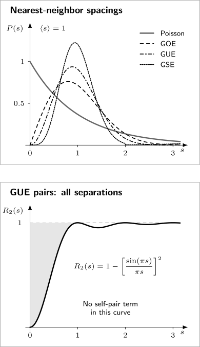
Nearest neighbors and arbitrary pairs answer different questions. Top: the normalized Poisson law and the three Wigner surmises, calculated from the displayed formulas. The latter approximate the large-matrix nearest-neighbor laws. Bottom: the exact unfolded bulk GUE pair correlator, excluding a level paired with itself. It vanishes at zero separation and tends to one, whereas every nearest-neighbor density decays at large spacing.

Spacing ratios

Define raw consecutive gaps and their symmetrized ratio by

$$\delta_n = E_{n+1}-E_n,$$ $$\widetilde r_n = \frac{ \min(\delta_n,\delta_{n+1}) }{ \max(\delta_n,\delta_{n+1}) }.$$

Because nearby gaps are rescaled by nearly the same smooth density, $\widetilde r_n$ often avoids explicit unfolding. For independent exponential gaps,

$$\left\langle \widetilde r \right\rangle_{\mathrm P} = 2\ln2-1 \simeq 0.38629.$$

Representative large-matrix values from Atas et al. (2013, Table I) are

Statistics	Mean $\widetilde r$
Poisson	$2\ln2-1\simeq0.38629$ (exact)
GOE	$\simeq0.5307$
GUE	$\simeq0.5996$
GSE, one level per pair	$\simeq0.6744$

For comparison with an analytic distribution, define the unsymmetrized ratio $r=\delta_{n+1}/\delta_n$. It can exceed one, whereas $\widetilde r=\min(r,1/r)$ lies between zero and one.

The compact ratio distribution

$$P_\beta(r) = \frac{1}{Z_\beta} \frac{ \left(r+r^2\right)^\beta }{ \left(1+r+r^2\right)^{1+3\beta/2} },$$

applies for $r\geq0$ and is itself a three-level surmise. Its means are close to the large-matrix numbers above but differ slightly: for example, the GOE surmise gives $4-2\sqrt3\simeq0.53590$. For these left-right symmetric spacing statistics, the density of $\widetilde r$ is $2P_\beta(\widetilde r)$ on $[0,1]$. A ratio average tests nearby gaps, not long-range rigidity.

Two-level correlations and the sine kernel

In the unfolded bulk of the GUE, the large-$N$ process is determinantal with kernel

$$K(s) = \frac{ \sin(\pi s) }{ \pi s }.$$

With mean density one, the normalized two-level correlation function for distinct levels is

$$R_2(s) = 1-K^2(s).$$

Thus

$$R_2(0) = 0, \qquad \lim_{\lvert s\rvert\to\infty} R_2(s) = 1.$$

The suppression near $s=0$ is the correlation hole. Unlike a nearest-neighbor density, $R_2$ includes pairs with other levels between them. It is not a normalized probability density over all separations: its limit is one, not zero. Including a level paired with itself adds the separate $\delta(s)$ term used below.

For the number $n_L$ of unfolded levels in an interval of length $L$, define the number variance

$$\Sigma^2(L) = \left\langle \left( n_L-L \right)^2 \right\rangle.$$

Poisson statistics give

$$\Sigma_{\mathrm P}^2(L) = L.$$

The Wigner–Dyson classes are much more rigid:

$$\Sigma_\beta^2(L) = \frac{2}{\beta\pi^2} \ln L + O(1), \qquad L\gg1.$$

Long-range statistics are more sensitive than ratios to imperfect unfolding, finite bandwidth, missing levels, and slow nonuniversal modes.

One connected GUE form-factor convention is

$$K_{\mathrm c}(\tau) = \int_{-\infty}^{\infty} ds\, e^{-2\pi i\tau s} \times \left[ \delta(s)+R_2(s)-1 \right].$$

It gives

$$K_{\mathrm c}(\tau) = \begin{cases} \lvert\tau\rvert, & \lvert\tau\rvert\leq1, \\ 1, & \lvert\tau\rvert\geq1. \end{cases}$$

The linear ramp and unit plateau follow only with this unfolding and normalization. Finite-temperature filters, disconnected pieces, finite observation windows, and many-body Thouless scales belong to the Many-Body Quantum Chaos Preview.

Wigner–Dyson classes

Resolve ordinary unitary symmetries first

Suppose a unitary operator $Q$ commutes with $H$. Then

$$\mathcal H = \bigoplus_q \mathcal H_q, \qquad H = \bigoplus_q H_q.$$

Random-matrix statistics must be computed within one irreducible block $H_q$. Momentum, parity, particle number, total spin, point-group representations, and gauge constraints can all produce independent sequences. An antiunitary symmetry may preserve a block, exchange two blocks, or square differently after internal structure is included; checking only the full Hamiltonian is insufficient.

The three bulk classes

After unitary block decomposition, the ordinary bulk classes are:

Class and ensemble	Antiunitary structure within the block
AI / GOE, $\beta=1$	A preserving antiunitary squares to $+I$.
A / GUE, $\beta=2$	No preserving antiunitary constraint.
AII / GSE, $\beta=4$	A preserving antiunitary squares to $-I$; count each Kramers pair once.

For a spinless Hamiltonian with a basis in which $\mathcal T=K$, time-reversal invariance permits a real symmetric representation and leads to class AI. Breaking the relevant antiunitary symmetry, for example with magnetic flux, gives class A. For half-integer spin with $\mathcal T^2=-I$ and no additional block exchange, Kramers degeneracy leads to class AII. Spin alone is insufficient: if spin rotation is conserved, a spin-independent Hamiltonian can reduce to two identical real orbital blocks with GOE statistics. Always test the antiunitary constraint on the block actually being analyzed.

These are symmetry statements, not statements about whether a material is literally orthogonal, unitary, or symplectic as a vector space. The labels name the transformation groups of the invariant ensemble.

Gaussian versus circular ensembles

Gaussian ensembles describe Hermitian spectra on the real line. For a unitary evolution operator,

$$U \lvert n\rangle = e^{-i\theta_n} \lvert n\rangle,$$

the eigenphases live on a circle. Circular ensembles have joint phase density

$$\mathcal P(\theta_1,\ldots,\theta_N) \propto \prod_{i<j} \left| e^{i\theta_i} - e^{i\theta_j} \right|^\beta.$$

The circular orthogonal, unitary, and symplectic ensembles share their local bulk limits with GOE, GUE, and GSE, respectively. They are natural for Floquet operators and scattering matrices because no artificial spectral edge is introduced. Floquet Operators develops quasienergy kinematics; Floquet Systems Preview treats driven many-body phases and heating.

Crossovers are parameter-dependent

A weak symmetry-breaking perturbation does not instantly replace one finite-size distribution by another. A crossover occurs when its typical matrix element becomes comparable with the local mean spacing. Schematically, if

$$H(\lambda) = H_{\mathrm{AI}} + \lambda V_{\mathrm{A}},$$

then the crossover parameter has the form

$$\Lambda \sim \frac{ \lambda^2 \overline{ \lvert V_{mn}\rvert^2 } }{ \Delta^2 }.$$

The precise coefficient depends on normalization. Reporting only the bare field or flux without $\Delta$, size, and symmetry sector obscures the scaling variable.

Level repulsion

Vandermonde Jacobian

Diagonalize

$$\begin{aligned} H&=U\Lambda U^{-1},\\ \Lambda&=\operatorname{diag}(\lambda_1,\ldots,\lambda_N). \end{aligned}$$

Changing variables from matrix entries to eigenvalues and eigenvectors produces the Jacobian

$$dH \propto \prod_{i<j} \lvert \lambda_i-\lambda_j \rvert^\beta \prod_i d\lambda_i\, d\mu(U).$$

After integrating over $U$,

$$\mathcal P(\boldsymbol\lambda) \propto \exp\!\left[ - \frac{\beta N}{4a^2} \sum_i\lambda_i^2 \right] \times \prod_{i<j} \lvert \lambda_i-\lambda_j \rvert^\beta.$$

The proportionality constant normalizes the joint density. The Vandermonde factor vanishes when two distinct levels coincide. Taking minus the logarithm turns that product into pair terms $-\beta\ln|\lambda_i-\lambda_j|$. These compete with the quadratic confining potential. This logarithmic-gas picture is an analogy for a joint probability density, not a literal force among energy levels.

Two-level avoided crossings

The local mechanism is visible without the full Jacobian. A real symmetric two-level Hamiltonian can be written

$$H_{\mathrm R} = E_0 I + x\sigma_z + v\sigma_x.$$

Its eigenvalues are

$$E_\pm = E_0 \pm \sqrt{x^2+v^2},$$

and the gap is

$$s \propto \sqrt{x^2+v^2}.$$

Near a degeneracy, the independent splitting coordinates form a two-dimensional vector. A smooth probability density assigns shell volume

$$dP \propto s^{2-1}\,ds,$$

which gives linear repulsion.

For a complex Hermitian two-level block,

$$H_{\mathrm C} = E_0I + x\sigma_x + y\sigma_y + z\sigma_z.$$

There are three splitting coordinates, so

$$dP \propto s^{3-1}\,ds = s^2\,ds.$$

The self-dual quaternionic problem has five independent splitting coordinates after Kramers pairing, giving

$$dP \propto s^{5-1}\,ds = s^4\,ds.$$

The splitting-coordinate count is $\beta+1$, so its radial shell volume gives $s^\beta\,ds$ in all three cases. This agrees with the Vandermonde Jacobian.

When exact crossings remain

Repulsion applies only between levels allowed to hybridize. Levels in different irreducible symmetry sectors can cross because their off-diagonal matrix element vanishes identically. Integrable systems can possess enough conserved structure to support crossings or uncorrelated sequences. Kramers partners remain exactly degenerate when $\mathcal T^2=-I$. Topological or chiral symmetry can pin eigenvalues at a special energy.

An observed crossing therefore asks two separate questions:

1. Is a coupling forbidden by an exact symmetry?
2. If not, is the apparent crossing unresolved because the gap lies below numerical or experimental resolution?

Quantum chaos

Spectral correspondences

For many generic classically integrable Hamiltonian systems, the Berry–Tabor correspondence predicts Poisson-like unfolded spectra in the semiclassical limit. For systems with a fully chaotic classical limit, the Bohigas–Giannoni–Schmit correspondence predicts the Wigner–Dyson class selected by antiunitary symmetry.

These statements have hypotheses and exceptions. Arithmetic systems, commensurate oscillators, mixed phase space, marginally stable orbits, unresolved discrete symmetries, and finite-energy effects can all alter the result. The Bohigas–Giannoni–Schmit statement is a highly successful universality conjecture, not a theorem covering every chaotic Hamiltonian.

Random-matrix agreement also does not define classical chaos. Unitary quantum evolution preserves the Hilbert-space distance between states evolved by the same operator. Classical sensitivity, periodic-orbit theory, Ehrenfest time, and eigenfunction scarring are developed in Quantum Chaos Preview.

An effective fluctuation theory

A local Hamiltonian is sparse in many useful bases and contains spatial structure that a dense Gaussian matrix lacks. Random-matrix agreement concerns selected correlations in a range of energy separations or times; it does not identify the two Hamiltonians entry by entry.

For a diffusive sample or local many-body system, let $t_{\mathrm{Th}}$ be the exploration or Thouless time,

$$E_{\mathrm{Th}} \sim \frac{\hbar}{t_{\mathrm{Th}}},$$

and let $\Delta$ be the mean level spacing. The dimensionless spectral conductance is

$$g_{\mathrm{Th}} \sim \frac{E_{\mathrm{Th}}}{\Delta}.$$

Random-matrix behavior is expected only below the system-dependent Thouless energy, or after the corresponding time, while microscopic, ballistic, hydrodynamic, and finite-size effects remain outside that window. Quantum Coherence in Conductors explains the competing dephasing, escape and thermal lengths.

Disorder and localization

In a disordered conductor, spectral statistics provide a compact spatial diagnostic:

In a diffusive metal, states hybridize across the coherent sample and can show Wigner–Dyson correlations below the Thouless energy. Localized states often have approximately Poisson spectra because distant orbitals overlap weakly. Anderson critical states have different scale-dependent correlations. Combine spectra with spatial localization tests or energy-resolved scaling: Poisson statistics alone cannot distinguish localization from integrability.

Symmetry classes and topology

The zero-dimensional tenfold extension

The three Wigner–Dyson classes assume no spectral symmetry that relates $E$ to $-E$. Superconducting and sublattice problems introduce two antiunitary possibilities and one unitary spectral symmetry:

$$\mathcal T H\mathcal T^{-1} = H,$$ $$\mathcal C H\mathcal C^{-1} = -H,$$ $$\mathcal S H\mathcal S^{-1} = -H.$$

Here $\mathcal T$ is time reversal, $\mathcal C$ is Altland–Zirnbauer particle–hole structure, and $\mathcal S$ is chiral symmetry. When both antiunitary symmetries exist, their product gives a chiral symmetry up to a phase. The complete tenfold classification organizes these constraints. Three useful examples beyond ordinary Wigner–Dyson statistics are:

Example	Constraint and spectral consequence
AIII	Chiral symmetry with neither antiunitary symmetry; nonzero energies occur in opposite pairs.
D	Particle–hole structure squares to $+I$, without time reversal; opposite-energy pairs and possible zero modes.
C	Particle–hole structure squares to $-I$, without time reversal; different correlations at zero energy.

These labels describe matrix constraints. They do not yet assign a spatial topological invariant.

In a Bogoliubov–de Gennes Hamiltonian, $\mathcal C$ usually expresses Nambu redundancy:

$$\mathcal C H_{\mathrm{BdG}}(\mathbf k) \mathcal C^{-1} = - H_{\mathrm{BdG}}(-\mathbf k).$$

It should not be confused with an ordinary many-body symmetry that exchanges physical particles and holes while preserving the Hamiltonian.

Special energy requires special statistics

Far from $E=0$, many chiral and superconducting ensembles recover an ordinary Wigner–Dyson bulk class. Near the symmetry point, however, eigenvalues occur in $\pm E$ pairs, exact zero modes may be present, and the density can have a hard edge or class-dependent singularity. The sine kernel and ordinary Wigner surmises are then not the correct complete benchmarks.

Near zero energy, the correct correlations depend on the symmetry class, protected zero modes and how Kramers or particle–hole partners are counted. A non-GOE histogram there can therefore agree with a different universal ensemble.

From ensemble class to topological phase

A free-fermion topological classification also needs spatial dimension, a bulk or mobility gap, allowed symmetry-preserving deformations and the convention for adding trivial bands. Topological Insulators and Topological Superconductors develop concrete invariants. Random-matrix statistics describe finite-volume fluctuations; they do not supply a bulk invariant by themselves.

Mesoscopic scattering

For a phase-coherent cavity attached to ideal leads, the on-shell scattering matrix satisfies

$$S^\dagger S = I.$$

When the dwell dynamics is sufficiently mixing, circular ensembles provide symmetry-controlled distributions for $S$. Observable conductance, shot noise, and delay times depend additionally on channel number, contact transparency, and transmission eigenvalues. What Is Mesoscopic Physics? gives the scale hierarchy; the scattering formulation should not be reduced to an energy-level histogram.

Exercises

1. Normalize the GOE Wigner surmise

Show that

$$P(s) = \frac{\pi}{2} s e^{-\pi s^2/4}$$

is normalized on $s\geq0$ and has unit mean.

Solution

For $a>0$,

$$\int_0^\infty s e^{-as^2}\,ds = \frac{1}{2a}.$$

With $a=\pi/4$,

$$\int_0^\infty P(s)\,ds = \frac{\pi}{2} \frac{1}{2(\pi/4)} = 1.$$

The mean uses

$$\int_0^\infty s^2e^{-as^2}\,ds = \frac{\sqrt{\pi}}{4a^{3/2}}.$$

Therefore

$$\begin{aligned} \langle s\rangle &= \frac{\pi}{2} \frac{\sqrt{\pi}}{ 4(\pi/4)^{3/2} } \\ &= 1. \end{aligned}$$

Normalization and unit mean fix the two constants in a trial form $As e^{-Bs^2}$.

2. Derive two-level repulsion

For

$$H = \begin{pmatrix} x & v \\ v & -x \end{pmatrix},$$

assume the joint density of $x$ and $v$ is smooth and nonzero at the origin. Derive the small-gap power law.

Solution

The eigenvalues are

$$E_\pm = \pm\sqrt{x^2+v^2},$$

so the gap is

$$g = 2\sqrt{x^2+v^2}.$$

Near the origin, use polar coordinates:

$$dx\,dv = r\,dr\,d\phi.$$

Because $g=2r$,

$$dP \propto r\,dr \propto g\,dg.$$

Hence

$$P(g) \propto g$$

at small $g$, the $\beta=1$ repulsion law. If $v$ is forced to zero by a symmetry, the radial argument collapses and an exact crossing at $x=0$ is allowed.

3. Unfold a nonuniform spectrum

Suppose three positive levels are

$$(E_1,E_2,E_3)=E_0(1,4,9),$$

and the smooth counting function is

$$\overline N(E) = \sqrt{\frac{E}{E_0}}.$$

Find the raw and unfolded gaps.

Solution

The raw gaps are

$$\delta E_1 = 3E_0, \qquad \delta E_2 = 5E_0.$$

The unfolded levels are

$$(\varepsilon_1,\varepsilon_2,\varepsilon_3)=(1,2,3).$$

Thus

$$s_1=s_2=1.$$

The increasing raw gaps came entirely from the decreasing smooth density. Treating them as changing correlations would be a false inference.

4. Derive the Poisson ratio mean

Let $x$ and $y$ be independent exponential gaps with density $e^{-x}$ for $x\geq0$. Show that

$$\widetilde r = \frac{\min(x,y)}{\max(x,y)}$$

has mean $2\ln2-1$.

Solution

By symmetry, integrate over $0\leq x\leq y$ and double:

$$\left\langle \widetilde r \right\rangle = 2 \int_0^\infty dy \int_0^y dx\, \frac{x}{y} e^{-x-y}.$$

Set $x=ry$, so $dx=y\,dr$:

$$\begin{aligned} \langle\widetilde r\rangle &=2\int_0^1 r I(r)\,dr,\\ I(r)&=\int_0^\infty y e^{-(1+r)y}\,dy. \end{aligned}$$

The inner integral is $1/(1+r)^2$, hence

$$\begin{aligned} \left\langle \widetilde r \right\rangle &= 2 \int_0^1 \frac{r}{(1+r)^2}\,dr \\ &= 2\ln2-1 \\ &\simeq 0.38629. \end{aligned}$$

5. Count Kramers pairs correctly

A finite class-AII spectrum is listed as

$$E_1,E_1,E_2,E_2,E_3,E_3.$$

What goes wrong if all six entries are used in a nearest-neighbor histogram, and what sequence should be analyzed?

Solution

Keeping all entries produces gaps

$$0,\, E_2-E_1,\, 0,\, E_3-E_2,\, 0.$$

The delta weight at zero is the exact Kramers degeneracy, not a failure of symplectic repulsion. Count each pair once and analyze

$$E_1,E_2,E_3,\ldots$$

within one otherwise irreducible block. The expected small-spacing law is then

$$P(s) \propto s^4.$$

References

• A. Altland and M. R. Zirnbauer, “Nonstandard Symmetry Classes in Mesoscopic Normal-Superconducting Hybrid Structures,” Physical Review B 55, 1142–1161 (1997), doi:10.1103/PhysRevB.55.1142. Completes the tenfold ensemble classification for normal and Bogoliubov–de Gennes systems.
• Y. Y. Atas, E. Bogomolny, O. Giraud, and G. Roux, “Distribution of the Ratio of Consecutive Level Spacings in Random Matrix Ensembles,” Physical Review Letters 110, 084101 (2013), doi:10.1103/PhysRevLett.110.084101. Derives practical spacing-ratio surmises and benchmark means.
• C. W. J. Beenakker, “Random-Matrix Theory of Quantum Transport,” Reviews of Modern Physics 69, 731–808 (1997), doi:10.1103/RevModPhys.69.731. Reviews circular ensembles, transmission eigenvalues, and mesoscopic transport.
• M. V. Berry and M. Tabor, “Level Clustering in the Regular Spectrum,” Proceedings of the Royal Society A 356, 375–394 (1977), doi:10.1098/rspa.1977.0140. Formulates the semiclassical Poisson correspondence for generic integrable systems.
• O. Bohigas, M.-J. Giannoni, and C. Schmit, “Characterization of Chaotic Quantum Spectra and Universality of Level Fluctuation Laws,” Physical Review Letters 52, 1–4 (1984), doi:10.1103/PhysRevLett.52.1. States the spectral-universality correspondence for classically chaotic systems.
• F. J. Dyson, “Statistical Theory of the Energy Levels of Complex Systems. I,” Journal of Mathematical Physics 3, 140–156 (1962), doi:10.1063/1.1703773. Develops invariant eigenvalue ensembles and the logarithmic-gas structure.
• F. J. Dyson, “The Threefold Way: Algebraic Structure of Symmetry Groups and Ensembles in Quantum Mechanics,” Journal of Mathematical Physics 3, 1199–1215 (1962), doi:10.1063/1.1703863. Establishes the orthogonal, unitary, and symplectic symmetry trichotomy.
• F. Evers and A. D. Mirlin, “Anderson Transitions,” Reviews of Modern Physics 80, 1355–1417 (2008), doi:10.1103/RevModPhys.80.1355. Reviews metallic, localized, and critical spectral statistics across localization classes.
• T. Guhr, A. Müller-Groeling, and H. A. Weidenmüller, “Random-Matrix Theories in Quantum Physics: Common Concepts,” Physics Reports 299, 189–425 (1998), doi:10.1016/S0370-1573(97)00088-4. Gives a broad account of correlation functions, universality, and physical applications.

Further Reading

• G. Akemann, J. Baik, and P. Di Francesco, eds., The Oxford Handbook of Random Matrix Theory, Oxford University Press, 2011, doi:10.1093/oxfordhb/9780198744191.001.0001. A broad reference spanning exact methods, universality, and applications.
• F. Haake, Quantum Signatures of Chaos, 3rd ed., Springer, 2010, doi:10.1007/978-3-642-05428-0. A systematic bridge from classical chaos to spectral and eigenfunction diagnostics.
• M. L. Mehta, Random Matrices, 3rd ed., Elsevier, 2004. A standard technical reference for invariant ensembles and correlation functions.