Quenches

A quantum quench is a controlled change of a Hamiltonian or state-preparation parameter on a timescale short compared with selected intrinsic dynamics, followed by time-resolved observation under the resulting generator. “Sudden” is therefore relative to a declared energy window. A pulse that is abrupt for collective modes may still be adiabatic for excluded electronic bands, while an ultrafast optical pump may populate those bands and invalidate a low-energy closed-system model.

The experimentally important questions are how much the state changes during the switch, which energies are populated, and what the subsequent signal measures. Quantum Quenches develops the exact evolution and worked models. Here we connect those ideas to calibrated ramps, propagation measurements and the limitations of a material’s effective Hamiltonian. Pump–Probe Spectroscopy treats the optical measurement in more detail.

Required background. Quantum Quenches supplies the state preparation, Hamiltonian switch and unitary-evolution framework. Relaxation and Thermalization supplies the distinction between transient relaxation and thermal agreement. Time-Dependent Correlations supplies operator ordering and two-time observables for specifying what the material probe measures.

Changing a material Hamiltonian in time

The preparation fixes the initial state; the waveform fixes the evolution during the switch. Both matter. A change in lattice depth, for example, can alter hopping and interactions simultaneously, while ringing can continue to drive the system after the nominal switch ends. Measure the waveform, its spatial variation and the relevant loss or heating before interpreting the late-time response.

Write a finite ramp as

$$H(t) = H_i + s(t) \left( H_f-H_i \right), \qquad s(0)=0, \qquad s(\tau_q)=1.$$

The actual post-ramp state is

$$|\psi(\tau_q)\rangle = \mathcal T \exp\!\left[ - \frac{i}{\hbar} \int_0^{\tau_q}H(t)\,dt \right] |\psi_0\rangle.$$

Only in an ideal sudden approximation is the state treated as unchanged during the switch:

$$|\psi(0^+)\rangle \approx |\psi(0^-)\rangle.$$

Replacing a measured waveform by an instantaneous step is a model assumption, not a definition.

Sudden for which degrees of freedom?

Suppose a low-energy model has a characteristic scale $\Delta_{\mathrm{IR}}$, while excluded states begin at $\Delta_{\mathrm{UV}}$ with $\Delta_{\mathrm{UV}}\gg\Delta_{\mathrm{IR}}$. A useful selective-quench window is

$$\frac{\hbar}{\Delta_{\mathrm{UV}}} \ll \tau_q \ll \frac{\hbar}{\Delta_{\mathrm{IR}}}.$$

This hierarchy is a useful scale estimate, not a complete adiabaticity test. The right inequality suppresses evolution on the retained slow scale. The left can suppress transitions to excluded states when the ramp is smooth, the relevant gap stays open and the coupling matrix elements are controlled.

For instantaneous states $|n(t)\rangle$ and $|m(t)\rangle$, a local adiabatic parameter is

$$\eta_{mn}(t)=\frac{\hbar|\langle m(t)|\dot H(t)|n(t)\rangle|}{|E_m(t)-E_n(t)|^2}.$$

Keeping this small for transitions out of the retained subspace is a useful diagnostic, together with the full ramp history. A small minimum gap, a large change in the eigenvectors or resonant spectral weight can invalidate an estimate based only on the final band gap. An optical pulse’s carrier frequency matters as well as its envelope duration.

No such window exists if the two scales are not separated. In that case one must simulate the finite ramp in a larger Hilbert space or weaken the claim.

Compare multiple ramp durations and, where practical, simulate the measured waveform in a space containing the nearest excluded states. This distinguishes a fast change within a model from excitation outside it. Spatially varying controls, avoided crossings, heating and residual periodic micromotion can each change the effective preparation.

Energy and work after the quench

After the switch, energy is conserved with respect to a time-independent isolated $H_f$, not $H_i$. For an ideal sudden switch, use the initial state; for a finite ramp, use the actual post-ramp state in the following expressions. The mean and variance are

$$\overline E_f = \langle\psi_0|H_f|\psi_0\rangle, \qquad \left(\Delta E_f\right)^2 = \langle H_f^2\rangle_0 - \overline E_f^{\,2}.$$

For a system of $N$ local degrees of freedom, define an excess-energy density relative to the final ground state:

$$\varepsilon_{\mathrm{ex}} = \frac{ \overline E_f-E_{0,f} }{N}.$$

For bounded lattice terms, a local switch $H_f=H_i+V$ with $\|V\|=O(1)$ changes the mean energy by at most $\|V\|$ in the sudden limit. A global change can instead do extensive work. Work can have either sign; excess energy above the final ground state is nonnegative.

These statements should not be confused with the energy already present in the preparation. If the initial state is the ground state of $H_i$, a local switch gives

$$0\leq\overline E_f-E_{0,f}\leq2\|V\|.$$

The bound follows from $|E_{0,f}-E_{0,i}|\leq\|V\|$ and $|\langle V\rangle_0|\leq\|V\|$. An initially thermal state can already have extensive energy above the ground state, even when the additional work is local. Unbounded continuum interactions need separate domain and energy-moment control.

Work in an isolated quench is not a Hermitian operator evaluated once. Under a two-projective-measurement protocol it is a random variable,

$$W = E_m^{f}-E_n^{i},$$

with probabilities determined by the first measurement and the ramp transition amplitudes. For a sudden switch from an initial energy eigenstate, those amplitudes reduce to overlaps of initial and final eigenstates (Silva, 2008).

The first energy measurement removes coherence between different initial energies. Consequently the two-measurement work statistics need not describe an otherwise unmeasured coherent preparation. Interferometric schemes must specify which characteristic function they reconstruct. Absorbed pump fluence is not automatically this work distribution; Quantum Quenches gives the precise definitions.

Return amplitudes and reversal experiments

For a pure initial state evolving under $H_f$, the Loschmidt amplitude and return probability are

$$\mathcal G(t) = \langle\psi_0| e^{-iH_ft/\hbar} |\psi_0\rangle, \qquad \mathcal L(t) = \left| \mathcal G(t) \right|^2.$$

Terminology varies: some authors call $\mathcal L$ a Loschmidt echo. Here return probability means projection back onto the initial state; reversal echo means a forward evolution followed by an attempted inverse. Describing the pulse sequence removes the ambiguity.

Quantity	Operational meaning
Return probability	Project the evolved state onto the initial state
Fidelity	Compare two declared states; conventions may square the overlap or not
Echo	Compare evolution under forward and imperfectly reversed generators
Ramsey or ancilla signal	Interferometrically reconstruct a complex amplitude
DQPT rate function	Take an intensive logarithm and examine its thermodynamic limit

A zero or cusp in a few-site return curve is not a thermodynamic dynamical phase transition. Loschmidt Echo and Dynamical Phase Transitions Preview explains the required size sequence, Fisher-zero structure and order of limits.

Relaxation after quenches

A quench defines a preparation, not its outcome. Coherent oscillations, generalized or ordinary thermalization, prethermal plateaus, localized memory and bath-driven relaxation are all possible (Polkovnikov et al., 2011).

The post-quench observable

$$\langle O(t)\rangle = \langle\psi_0| e^{iH_ft/\hbar} O e^{-iH_ft/\hbar} |\psi_0\rangle$$

must be interpreted with conserved quantities and finite-size timescales. If

$$[H_f,\rho_0] = 0,$$

then every time-independent Schrödinger-picture observable has a stationary expectation value even if $H_i\ne H_f$. State evolution requires $[H_f,\rho_0]\ne0$: the preparation must contain coherence between distinct final energies. Unequal populations alone do not suffice; a density matrix diagonal in the final energy basis remains stationary, whatever those populations are. Whether a particular observable changes also depends on its matrix elements.

Quantum Thermalization supplies the positive ensemble test after relaxation. A smooth trace alone establishes neither thermalization nor irreversibility.

Correlation fronts and locality

For bounded local operators $A_x$ and $B_y$ separated by distance $r$, finite-range spin Hamiltonians with uniformly bounded interactions satisfy a Lieb–Robinson-type bound (Lieb and Robinson, 1972)

$$\left\| \left[ A_x(t),B_y \right] \right\| \le C \exp\!\left[ - \mu \left( r-v_{\mathrm{LR}}|t| \right) \right].$$

This bounds an unequal-time commutator and hence the response to a local perturbation. It gives an exponentially small tail outside a propagation region, not an exact zero or a unique measured velocity. Peak, onset, operator-growth and entanglement velocities need not coincide. Unbounded bosonic models and long-range interactions require additional assumptions or modified bounds.

An equal-time correlation after a global quench is a different object. In a ballistic quasiparticle picture, the quench creates correlated partners that move apart with velocities $v_1$ and $v_2$. Their separation grows as $|v_1-v_2|t$. Oppositely moving partners at $\pm v$ therefore correlate sites separated by $2vt$, although each travels only $vt$ (Calabrese and Cardy, 2006; Cheneau et al., 2012).

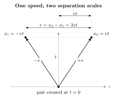
One correlated pair created by a global quench: each partner travels at speed $v$, while the separation relevant to an equal-time two-point correlation grows at $2v$. The diagram illustrates the ballistic pair picture; a general interacting system need not have sharp quasiparticles or this exact front.

Initial correlations also matter. To interpret a new correlation cone, account for the correlations already present before the switch; locality alone does not remove long-range correlations in the initial state. Bravyi, Hastings and Verstraete (2006) relate correlation growth bounds to initially short-ranged correlations. Specify whether the horizontal coordinate is distance from a local source or separation between two detectors before comparing a front with a band velocity.

Cold atoms, ions and qubit arrays

Platform	Switch, probe and leading limitation
Optical-lattice atoms	Change lattice depth or interactions; measure density and correlations; check trapping, ramp excitations and loss.
One-dimensional gases	Split, join or change confinement; measure correlations and momentum; account for tube averaging and near-integrability.
Trapped-ion spins	Change fields or couplings; measure spatial spin correlations; include interaction range and inhomogeneity.
Superconducting qubits	Change a programmed Hamiltonian or detuning; measure tomography or return; characterize gate errors and decoherence.

Cold-atom quenches can approximate closed-system unitary evolution over a broad window. Their principal advantage is not perfect isolation but the ability to measure loss and dephasing independently and compare them with the intrinsic timescale.

The collapse-and-revival experiment of Greiner et al. (2002) in an optical lattice is a useful warning against equating collapse with irreversible relaxation. Discrete interaction phases can rephase, revealing coherent finite-system dynamics.

The measured correlation front after a Bose–Hubbard quench provides a spatial diagnostic stronger than a one-point decay: it tests propagation, velocity, and quasiparticle structure together.

Pump–probe quenches in solids

An ultrafast pump can change occupations, screening, lattice coordinates and effective interactions at the same time. Its delayed probe samples a response that also depends on optical matrix elements and penetration depth. There may be no interval with a time-independent isolated final Hamiltonian: electrons, phonons and the substrate can exchange energy throughout the measurement (Giannetti et al., 2016).

A gap-like feature demonstrates changed spectral weight in the measured window; it does not by itself identify a homogeneous equilibrium phase. Coherent oscillations can originate in driven lattice or collective modes. Compare absorbed energy, relaxation channels and independent probes of the proposed order before interpreting a transient resemblance to an equilibrium spectrum. Pump–Probe Spectroscopy develops these comparisons.

Exercises

1. A selective suddenness window

A low-energy mode has $\Delta_{\mathrm{IR}}=20\ \mathrm{meV}$ and excluded bands begin at $\Delta_{\mathrm{UV}}=5.0\ \mathrm{eV}$. Using $\hbar=0.658\ \mathrm{eV\,fs}$, test whether a $5\ \mathrm{fs}$ switch lies in the selective-quench window.

Solution

The two inverse-energy times are

$$\frac{\hbar}{\Delta_{\mathrm{UV}}} = \frac{0.658}{5.0}\ \mathrm{fs} \approx 0.132\ \mathrm{fs},$$

and

$$\frac{\hbar}{\Delta_{\mathrm{IR}}} = \frac{0.658}{0.020}\ \mathrm{fs} \approx 32.9\ \mathrm{fs}.$$

Thus

$$0.132\ \mathrm{fs} < 5\ \mathrm{fs} < 32.9\ \mathrm{fs}.$$

The dimensionless estimates are $\tau_q\Delta_{\mathrm{IR}}/\hbar\simeq0.152$ and $\hbar/(\tau_q\Delta_{\mathrm{UV}})\simeq0.0263$. The switch lies between the two timescales, but the first ratio is not extremely small. This motivates a finite-ramp correction rather than establishing a precise sudden approximation. Excluded-band populations still depend on matrix elements, minimum gaps and pulse spectrum.

2. Local versus global injection

A local quench changes one bond by $\delta J$, while a global quench changes every one of $N$ bonds by the same amount. How do their injected energies scale generically?

Solution

For bounded bond operators, the local perturbation norm is order $|\delta J|$, so the magnitude of the additional sudden work is bounded independently of $N$. Its contribution per site vanishes as $N^{-1}$. The initial energy density need not vanish.

The global perturbation is a sum of $N$ bounded local changes, so its norm can scale as $N|\delta J|$. It can therefore change the energy density by a finite amount. This is a scaling allowance, not a lower bound: symmetries or a special initial state can suppress the work. For initial ground states, the final excess-energy density is generically finite after a global quench and vanishes after a local one.

3. A quench with no dynamics

Show why a state satisfying $[H_f,\rho_0]=0$ remains stationary after the switch.

Solution

The evolved state is

$$\rho(t) = e^{-iH_ft/\hbar} \rho_0 e^{iH_ft/\hbar}.$$

If $\rho_0$ commutes with $H_f$, it also commutes with every function of $H_f$, so

$$\rho(t) = \rho_0.$$

Every time-independent observable has a stationary expectation value. The Hamiltonian may have changed, but the prepared state has no coherence between distinct final energies. Unequal diagonal populations, or coherence confined to a degenerate energy subspace, do not change this conclusion.

4. Which front velocity?

A global quench creates counterpropagating pairs with maximum single-particle speed $v_{\max}=2.4Ja/\hbar$. A correlation map plotted against detector separation has onset near $r/t=3Ja/\hbar$ and a ridge near $2Ja/\hbar$. Do these numbers violate the quasiparticle picture?

Solution

The largest pair-separation speed in this symmetric ballistic model is $2v_{\max}=4.8Ja/\hbar$. Both measured values lie below it. The onset and ridge can differ because the experiment weights momenta differently and detects tails only above a threshold. Neither is automatically the single-particle group velocity or the Lieb–Robinson bound parameter.

If the experiment instead perturbs one localized source and measures its response at distance $r$, the relevant ballistic comparison is $v_{\max}$, not $2v_{\max}$. A persistent asymptotic response front above that model’s maximum speed would require checking the dispersion, interactions, model assumptions and signal definition; a threshold fit at short times alone cannot settle it.

References

• S. Bravyi, M. B. Hastings, and F. Verstraete, “Lieb–Robinson Bounds and the Generation of Correlations and Topological Quantum Order,” Physical Review Letters 97, 050401 (2006), doi:10.1103/PhysRevLett.97.050401. Connects locality bounds to correlation and entanglement growth.
• P. Calabrese and J. Cardy, “Time Dependence of Correlation Functions Following a Quantum Quench,” Physical Review Letters 96, 136801 (2006), doi:10.1103/PhysRevLett.96.136801. Develops the quasiparticle and light-cone picture in one-dimensional critical systems.
• M. Cheneau et al., “Light-Cone-Like Spreading of Correlations in a Quantum Many-Body System,” Nature 481, 484–487 (2012), doi:10.1038/nature10748. Measures a propagating correlation front after a Bose–Hubbard quench.
• C. Giannetti et al., “Ultrafast Optical Spectroscopy of Strongly Correlated Materials and High-Temperature Superconductors: A Non-Equilibrium Approach,” Advances in Physics 65, 58–238 (2016), doi:10.1080/00018732.2016.1194044. Reviews pump–probe modeling, coupled relaxation channels, and the interpretation of transient states.
• M. Greiner, O. Mandel, T. W. Hänsch, and I. Bloch, “Collapse and Revival of the Matter Wave Field of a Bose–Einstein Condensate,” Nature 419, 51–54 (2002), doi:10.1038/nature00968. Demonstrates coherent interaction-driven collapse and revival after a lattice-depth jump.
• E. H. Lieb and D. W. Robinson, “The Finite Group Velocity of Quantum Spin Systems,” Communications in Mathematical Physics 28, 251–257 (1972), doi:10.1007/BF01645779. Establishes the foundational locality bound.
• A. Polkovnikov, K. Sengupta, A. Silva, and M. Vengalattore, “Colloquium: Nonequilibrium Dynamics of Closed Interacting Quantum Systems,” Reviews of Modern Physics 83, 863–883 (2011), doi:10.1103/RevModPhys.83.863. Reviews quench protocols, methods, and nonequilibrium regimes.
• A. Silva, “Statistics of the Work Done on a Quantum Critical System by Quenching a Control Parameter,” Physical Review Letters 101, 120603 (2008), doi:10.1103/PhysRevLett.101.120603. Connects quench work statistics and return amplitudes.

Further Reading

• P. Calabrese and J. Cardy, “Quantum Quenches in Extended Systems,” Journal of Statistical Mechanics: Theory and Experiment 2007, P06008 (2007), doi:10.1088/1742-5468/2007/06/P06008. A foundational field-theory treatment.
• M. A. Cazalilla and M. Rigol, “Focus on Dynamics and Thermalization in Isolated Quantum Many-Body Systems,” New Journal of Physics 12, 055006 (2010), doi:10.1088/1367-2630/12/5/055006. An overview of experimental and theoretical directions.