London Theory

London theory relates a supercurrent to the gauge-invariant momentum of a phase-coherent charged fluid. In its simplest form it predicts magnetic screening over a penetration depth $\lambda_L$. The theory assumes local, linear response and a nearly fixed order-parameter amplitude; it does not determine the pairing mechanism or resolve a vortex core.

The central distinction is between perfect conductivity, which can preserve an initially trapped magnetic field, and the equilibrium Meissner response, which screens a weak applied field. Geometry matters: a thin slab admits substantial field, while a ring can carry a quantized fluxoid without containing an integer number of magnetic flux quanta.

Required background. Classical Electromagnetism supplies Maxwell boundary conditions; Minimal Coupling in Wave Mechanics supplies the signed-charge momentum. Helpful background. Gauge Transformations explains the compensating phase and potential changes.

Superfluid density and London electrodynamics

Use SI units and a nonmagnetic background, so the magnetic-field energy is $B^2/(2\mu_0)$. Let $q^\ast$ be the signed charge of the coherent object, $m^\ast$ its inertial parameter, and $n_s$ its density in that convention. For Cooper pairs, $q^\ast=-2e$ with $e>0$. Pair density, pair mass and pair charge must be used together. Counting superconducting electrons instead gives the same electromagnetic stiffness only when all three quantities are converted consistently.

Define

$$D_s=\frac{n_s(q^\ast)^2}{m^\ast}, \qquad \lambda_L^{-2}=\mu_0D_s.$$

In a crystal, $D_s$ is a response coefficient, generally a tensor. It need not equal the total carrier density times the bare charge-to-mass combination. A measured penetration depth therefore measures stiffness; it is not a model-independent count of paired electrons.

Writing a coarse-grained field as $\Psi=\sqrt{n_s}e^{i\theta}$ is a convenient normalization of this phenomenological model. It does not identify its amplitude with the largest eigenvalue of a microscopic density matrix. Off-Diagonal Long-Range Order explains that separate coherence diagnostic.

Gauge-invariant condensate momentum

Minimal coupling gives

$$\begin{aligned} \mathbf p_s&=\hbar\boldsymbol\nabla\theta-q^\ast\mathbf A,\\ \mathbf j_s&=\frac{n_sq^\ast}{m^\ast}\mathbf p_s. \end{aligned}$$

Under $\mathbf A\mapsto\mathbf A+\boldsymbol\nabla\chi$ and $\theta\mapsto\theta+q^\ast\chi/\hbar$, the two added gradients cancel in $\mathbf p_s$. The current is gauge invariant. The abbreviated relation $\mathbf j_s=-D_s\mathbf A$ requires a compatible constant-phase choice; it is not the general constitutive law.

For uniform scalar stiffness, the London free energy is

$$\begin{aligned} F_L&=F_{\rm matter}+F_B,\\ F_{\rm matter}&=\int d^3r\,\frac{n_s|\mathbf p_s|^2}{2m^\ast},\\ F_B&=\int d^3r\,\frac{|\mathbf B|^2}{2\mu_0}. \end{aligned}$$

Varying the matter term with respect to $\mathbf A$ gives $-\mathbf j_s$. Varying the entire functional instead gives

$$\frac{\delta F_L}{\delta\mathbf A} =-\mathbf j_s+\frac{\boldsymbol\nabla\times\mathbf B}{\mu_0}.$$

Its stationarity is magnetostatic Ampère law, with the external field imposed through boundary conditions. It does not require the screening current to vanish.

Away from vortices, $\boldsymbol\nabla\times\boldsymbol\nabla\theta=0$. Taking the curl of the current gives the second London equation:

$$\boldsymbol\nabla\times\mathbf j_s=-D_s\mathbf B.$$

The first London equation, $\partial_t\mathbf j_s=D_s\mathbf E$, describes acceleration in the uniform transverse response, with fixed stiffness and no additional electrochemical-potential gradient. A general longitudinal problem also needs phase dynamics, compressibility and charge conservation. Integrating the first equation with Faraday’s law leaves a history-dependent integration constant; the second equation selects the Meissner relation.

Meissner screening

Combining $\boldsymbol\nabla\times\mathbf B=\mu_0\mathbf j_s$ with the second London equation and $\boldsymbol\nabla\cdot\mathbf B=0$ yields

$$\nabla^2\mathbf B=\frac{\mathbf B}{\lambda_L^2}.$$

Half-space

For a superconductor in $x>0$ with a parallel boundary field $B_z(0)=B_0$, boundedness at large $x$ selects

$$\begin{aligned} B_z(x)&=B_0e^{-x/\lambda_L},\\ j_{s,y}(x)&=-\frac{1}{\mu_0}\frac{dB_z}{dx},\\ &=\frac{B_0e^{-x/\lambda_L}}{\mu_0\lambda_L},\\ K_y&=\int_0^\infty j_{s,y}(x)\,dx =\frac{B_0}{\mu_0}. \end{aligned}$$

The surface current of elementary magnetostatics is distributed over a finite layer. Its kinetic energy density $\mu_0\lambda_L^2j_s^2/2$ equals the magnetic energy density $B^2/(2\mu_0)$ point by point in this ideal solution.

A finite slab

For $-d/2\le x\le d/2$, with equal parallel fields $B_a$ at the faces, reflection symmetry selects a cosh profile:

$$\begin{aligned} \frac{B_z(x)}{B_a} &=\frac{\cosh(x/\lambda_L)}{\cosh[d/(2\lambda_L)]},\\ \frac{\langle B_z\rangle}{B_a} &=\frac{2\lambda_L}{d}\tanh\frac{d}{2\lambda_L}. \end{aligned}$$

When $d\gg\lambda_L$, most of the interior is field free. When $d\ll\lambda_L$, nearly all the field penetrates. This weak screening of a parallel field does not imply a vanishing superconducting stiffness.

A reversible Meissner state reaches the same equilibrium configuration whether a weak field is applied before or after cooling. A perfect conductor alone instead preserves initial flux. Real superconductors can retain flux through vortices, pinning or metastable barriers; field history and equilibration must therefore be considered when interpreting a screening measurement.

Fluxoid quantization in a ring

Along a closed contour where $\Psi\ne0$, single-valuedness gives $\oint\boldsymbol\nabla\theta\cdot d\boldsymbol\ell=2\pi w$, with integer $w$. Integrating the momentum relation gives

$$\begin{aligned} \Phi_f-\Phi&=\mu_0\lambda_L^2\oint\mathbf j_s\cdot d\boldsymbol\ell,\\ \Phi_f&=w\frac{h}{q^\ast}=n\Phi_0, \end{aligned}$$

where

$$\begin{aligned} \Phi&=\int_{\mathcal S}\mathbf B\cdot d\mathbf S,\\ n&=\operatorname{sgn}(q^\ast)w,\\ \Phi_0&=\frac{h}{|q^\ast|}. \end{aligned}$$

For Cooper pairs, $\Phi_0=h/(2e)\simeq2.068\times10^{-15}\,\mathrm{Wb}$. The signed winding $w$ and positive-quantum integer $n$ differ by a minus sign for negatively charged pairs.

The fluxoid $\Phi_f$ includes the current term. Flux itself is approximately $n\Phi_0$ only if the contour can be taken deep inside a thick wall where the current is negligible. In a simply connected, nonsingular Meissner region, a loop shrinks to a point and $w=0$.

For a narrow ring with uniform current across wire area $A_w$ and circumference $\ell$, define its kinetic inductance

$$L_k=\mu_0\lambda_L^2\frac{\ell}{A_w}.$$

If $L_g$ is the geometric inductance and $\Phi_{\rm ext}$ the applied flux, the lumped model gives

$$\begin{aligned} \Phi&=\Phi_{\rm ext}+L_g I,\\ \Phi+L_kI&=n\Phi_0,\\ I&=\frac{n\Phi_0-\Phi_{\rm ext}}{L_g+L_k}. \end{aligned}$$

Increasing $L_k/L_g$ allows flux to depart substantially from $n\Phi_0$ while the fluxoid remains quantized. These equations describe a chosen winding branch; a phase slip can change $n$. They also require currents below the scale that strongly suppresses the amplitude.

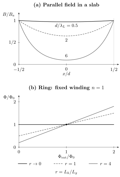
Geometry changes London screening. Above: slabs with different $d/\lambda_L$ have the same boundary field but different interior fields. Below: on the fixed $n=1$ ring branch, $\Phi/\Phi_0=(1+r f)/(1+r)$, where $r=L_k/L_g$ and $f=\Phi_{\rm ext}/\Phi_0$. The horizontal curve is the $L_k/L_g\to0$ limit. The figure does not assume that this branch is the equilibrium state at every applied flux.

Thin films and the Pearl scale

For a film with $d\ll\lambda_L$, a perpendicular vortex or a laterally varying field produces currents that are nearly uniform through the thickness, while stray fields spread into the surrounding vacuum. The crossover distance in the plane is

$$\Lambda_P=\frac{2\lambda_L^2}{d}.$$

Some authors call $\lambda_L^2/d$ the Pearl length, so its definition must accompany a number. In Pearl’s thin-film solution, the isolated-vortex sheet current changes from a $1/r$ dependence for $\xi\ll r\ll\Lambda_P$ to $1/r^2$ for $r\gg\Lambda_P$. This perpendicular-field geometry differs from the parallel-field slab solved above. See Vortices for core cutoffs and interactions.

Frequency-domain response and dissipative screening

Use $e^{-i\omega t}$ time dependence. The causal London conductivity is

$$\begin{aligned} \sigma_s(\omega)&=\frac{iD_s}{\omega+i0^+},\\ \operatorname{Re}\sigma_s&=\pi D_s\delta(\omega),\\ \operatorname{Im}\sigma_s&=D_s\,\mathcal P\frac1\omega. \end{aligned}$$

Here $\mathcal P$ is the principal value. The reactive pole and zero-frequency absorption weight are two parts of the same causal response. At finite frequency, quasiparticles add a regular conductivity $\sigma_n$; vortex motion can add another response if the sample is not in the Meissner state.

The sign of a complex penetration length must be tied to its decaying field solution. Neglect displacement current and write $B_z(x)=B_0e^{-q x}$ in $x>0$. Maxwell’s equations give

$$\begin{aligned} q^2&=-i\mu_0\omega\sigma,\\ \sigma&=\sigma_n+\frac{iD_s}{\omega},\\ q^2&=\lambda_L^{-2}-i\mu_0\omega\sigma_n,\\ \widetilde\lambda&=q^{-1},\qquad \operatorname{Re}q>0. \end{aligned}$$

For positive frequency and real positive $\sigma_n$, this branch has $\operatorname{Im}\widetilde\lambda>0$. Defining the surface impedance for these field directions gives

$$\begin{aligned} Z_s&=\frac{E_y(0)}{H_z(0)}=\frac q\sigma,\\ &=-i\mu_0\omega\widetilde\lambda,\\ Z_s&=R_s-iX_s. \end{aligned}$$

The dissipated surface power per area is $R_s|H_z(0)|^2/2\ge0$. A lossless London fluid has $Z_s=-i\mu_0\omega\lambda_L$; an ordinary Ohmic conductor instead has

$$\begin{aligned} \widetilde\lambda&=\frac{1+i}{2}\delta,\\ \delta&=\sqrt{\frac{2}{\mu_0\omega\sigma_n}},\\ Z_s&=(1-i)\sqrt{\frac{\mu_0\omega}{2\sigma_n}}. \end{aligned}$$

Using $e^{+i\omega t}$ conjugates these signs. A microwave penetration depth is therefore not automatically the static $\lambda_L$. Terahertz and Infrared Probes connects complex conductivity to measured spectra and missing-area tests.

Penetration depth as a material observable

A useful dimensionless stiffness ratio is $r_s(T)=\lambda_L^2(0)/\lambda_L^2(T)$. In the clean, local, isotropic, fully gapped weak-coupling limit,

$$\frac{\Delta\lambda_L(T)}{\lambda_L(0)} \simeq\sqrt{\frac{\pi\Delta_0}{2k_{\mathrm B}T}} \,e^{-\Delta_0/(k_{\mathrm B}T)}.$$

Nodes can give power laws, but the exponent also depends on the current direction and its matrix element near the node. For example, simple clean axial point-node models can give $T^2$ or $T^4$ in different directions; polar line-node models can give $T$ or $T^3$. Disorder, nonlocality and surface states further change the result. A single fitted power is not a unique identification of gap symmetry (Prozorov and Giannetta, 2006).

For anisotropic local response, replace $D_s$ by a tensor $\mathsf D$; the inverse squared penetration-depth tensor is $\mu_0\mathsf D$. Field direction, current direction and sample shape are needed to solve the screening problem. Independent-band models add band contributions, but general multiband response can also contain interband current terms.

Microwave impedance, resonators, mutual inductance, muon measurements and scanning magnetic probes infer stiffness through different field models. Many determine $\lambda(T)-\lambda(T_{\rm base})$ more accurately than absolute $\lambda(0)$. Calibration, demagnetization, trapped vortices and normal-fluid loss must be included before comparing the result with a gap model. Unconventional Superconductivity combines this information with other probes.

When the local model fails

If the current samples the vector potential over distances comparable to the field-variation scale, a nonlocal kernel replaces the pointwise law. Schematically,

$$j_i(\mathbf r)=\int d^3r'\, \mathcal K_{ij}(\mathbf r,\mathbf r')p_{s,j}(\mathbf r').$$

This is the setting of Pippard electrodynamics. The local limit requires a kernel range small compared with the electromagnetic variation, not merely a low frequency.

Strong currents, pair-breaking surfaces and vortex cores also violate the fixed-amplitude approximation. Ginzburg–Landau Theory introduces amplitude healing and critical scales; BCS Theory connects pairing to microscopic response. London theory can estimate a vortex’s far-field energy and, with additional core information, a lower critical field. Stiffness alone cannot determine the core energy, transition temperature, gap symmetry or type-I/type-II boundary.

Exercises

1. Weak screening in a thin slab

Derive the slab profile and its mean field, then obtain the leading small-$d/\lambda_L$ reduction of the mean field.

Solution

The general solution is $B=C\cosh(x/\lambda_L)+D\sinh(x/\lambda_L)$. Equal fields at both faces set $D=0$ and $C=B_a/\cosh[d/(2\lambda_L)]$. Integrating across the thickness gives the mean displayed above. With $a=d/(2\lambda_L)$,

$$\begin{aligned} \frac{\langle B\rangle}{B_a}&=\frac{\tanh a}{a} =1-\frac{a^2}{3}+O(a^4),\\ 1-\frac{\langle B\rangle}{B_a}&=\frac{d^2}{12\lambda_L^2} +O(d^4/\lambda_L^4). \end{aligned}$$

Thus the parallel-field diamagnetic response is small even for a perfectly coherent thin slab.

2. A ring with large kinetic inductance

Take $L_g=10\,\mathrm{pH}$, $L_k=90\,\mathrm{pH}$, $\Phi_{\rm ext}=0$ and winding branch $n=1$. Find $I$ and $\Phi$. Check them by minimizing the magnetic plus kinetic energy at fixed external flux.

Solution

$$\begin{aligned} I&=\frac{\Phi_0}{100\,\mathrm{pH}} \simeq20.68\,\mu\mathrm A,\\ \Phi&=L_gI=0.1\Phi_0. \end{aligned}$$

For general $n$ and external flux, the two inductive energies are

$$E(\Phi)=\frac{(\Phi-\Phi_{\rm ext})^2}{2L_g} +\frac{(n\Phi_0-\Phi)^2}{2L_k}.$$

Setting its derivative to zero gives

$$\Phi=\frac{L_k\Phi_{\rm ext}+L_gn\Phi_0}{L_g+L_k}.$$

At zero applied flux, $n=0$ has lower energy; the stated $n=1$ solution is a possible trapped branch, provided a phase-slip barrier and a sufficiently low current support it. Quantization constrains the fluxoid even though this branch contains only one tenth of a flux quantum of magnetic flux.

3. Where does the absorbed power go?

For $B_z=B_0e^{-q x}$ and real $\sigma_n>0$, show that the surface power equals the integrated quasiparticle Joule heating. Use $e^{-i\omega t}$.

Solution

Write $q=a-ib$ with $a>0$. From $q^2=\lambda_L^{-2}-i\mu_0\omega\sigma_n$,

$$2ab=\mu_0\omega\sigma_n.$$

Also $E_y(x)=Z_s H_z(0)e^{-q x}$. Therefore

$$\begin{aligned} \frac{P_{\rm bulk}}{A} &=\frac{\sigma_n}{2}\int_0^\infty|E_y|^2dx\\ &=\frac{\sigma_n|Z_sH_z(0)|^2}{4a}. \end{aligned}$$

Since $Z_s=-i\mu_0\omega/q$, its real part is $R_s=\mu_0\omega b/(a^2+b^2)>0$. Substituting $2ab=\mu_0\omega\sigma_n$ gives $P_{\rm bulk}/A=R_s|H_z(0)|^2/2$. Reversing the imaginary sign of $\widetilde\lambda$ without changing the time convention would incorrectly predict negative absorption.

4. Two screening questions for one film

A film has $d=20\,\mathrm{nm}$ and $\lambda_L=200\,\mathrm{nm}$. Estimate the mean parallel-field reduction and the Pearl scale. Why are these different questions?

Solution

The slab result gives $1-\langle B\rangle/B_a\simeq0.1^2/12=8.33\times10^{-4}$. For a perpendicular vortex or laterally varying field,

$$\Lambda_P=\frac{2(200\,\mathrm{nm})^2}{20\,\mathrm{nm}} =4.0\,\mu\mathrm m.$$

The first result concerns variation through the thickness; the second concerns currents and stray fields over lateral distances. Neither can replace the other by substituting a single sample dimension.

References

• B. S. Deaver, Jr. and W. M. Fairbank, “Experimental evidence for quantized flux in superconducting cylinders,” Physical Review Letters 7, 43–46 (1961), doi:10.1103/PhysRevLett.7.43.
• F. London and H. London, “The electromagnetic equations of the supraconductor,” Proceedings of the Royal Society A 149, 71–88 (1935), doi:10.1098/rspa.1935.0048.
• J. Pearl, “Current distribution in superconducting films carrying quantized fluxoids,” Applied Physics Letters 5, 65–66 (1964), doi:10.1063/1.1754056.
• A. B. Pippard, “An experimental and theoretical study of the relation between magnetic field and current in a superconductor,” Proceedings of the Royal Society A 216, 547–568 (1953), doi:10.1098/rspa.1953.0040.
• R. Prozorov and R. W. Giannetta, “Magnetic penetration depth in unconventional superconductors,” Superconductor Science and Technology 19, R41–R67 (2006), doi:10.1088/0953-2048/19/8/R01.
• M. Tinkham, Introduction to Superconductivity, 2nd ed., Dover (2004).