Ginzburg–Landau Theory

Ginzburg–Landau (GL) theory describes how a superconducting amplitude varies in space and responds to fields and currents. Unlike the fixed-amplitude London model, it can describe a suppressed surface, a vortex core and the loss of superconductivity through orbital magnetic coupling. Its simplest controlled setting is a local, single-component order parameter near a continuous transition, outside the region where strong fluctuations invalidate mean-field minimization.

The essential competition is between condensation energy, amplitude gradients and magnetic-field energy. It produces an amplitude scale $\xi$, a screening length $\lambda$ and the ratio $\kappa=\lambda/\xi$. These quantities organize the distinction between type-I and type-II behavior in the minimal bulk model.

Required background. London Theory supplies gauge-invariant current and screening; Landau–Ginzburg Theory supplies free-energy minimization and fluctuation limits. Helpful background. Minimal Coupling explains the covariant momentum operator.

A charged order parameter and its free energy

Use SI units, a nonmagnetic background and the signed pair charge $q^\ast=-2e$, with $e>0$. Define

$$\boldsymbol\Pi=-i\hbar\boldsymbol\nabla-q^\ast\mathbf A, \qquad \mathbf B=\boldsymbol\nabla\times\mathbf A.$$

For one isotropic complex field, the free energy relative to the zero-field normal reference is

$$\begin{aligned} F&=\int_\Omega d^3r\,[f_{\rm pot}+f_{\rm grad}+f_B],\\ f_{\rm pot}&=\alpha|\psi|^2+\frac\beta2|\psi|^4,\\ f_{\rm grad}&=\frac{|\boldsymbol\Pi\psi|^2}{2m^\ast},\\ f_B&=\frac{B^2}{2\mu_0}. \end{aligned}$$

The local potential favors either zero or nonzero amplitude; gradients penalize spatial variation and coherent flow; the last term accounts for the magnetic field. We take $\beta>0$ and

$$\alpha(T)=\alpha_0(T-T_c),\qquad\alpha_0>0,$$

with $\beta$ and $m^\ast$ smooth near $T_c$. This is a near-transition expansion, not a prescribed temperature dependence down to absolute zero.

The normalization $|\psi|^2=n_s$ is convenient, but $\psi$ is a collective field, not a literal two-electron wavefunction. Rescaling $\psi$ changes the coefficients without changing observables. Its electromagnetic stiffness is what can be measured directly; identifying its amplitude with a microscopic condensate population requires a derivation.

Under $\psi\mapsto e^{iq^\ast\chi/\hbar}\psi$ and $\mathbf A\mapsto\mathbf A+\boldsymbol\nabla\chi$, the energy is unchanged. Observable statements concern amplitude, currents, magnetic fields and covariant phase differences. A gauge redundancy is not an observable global symmetry that literally breaks; see Phase Symmetry and Gauge Theory.

Which magnetic energy should be minimized?

The displayed functional includes internal field energy. At fixed applied field $\mathbf H_a$, the Gibbs functional contains the additional term $-\int\mathbf H_a\cdot\mathbf B\,d^3r$, together with the appropriate exterior-field problem. For an ideal bulk sample with negligible demagnetization, this term permits equilibrium comparison at a specified $H_a$. For a finite specimen, stray fields and shape must also be solved. A magnetic onset field cannot be interpreted without this geometry.

Uniform equilibrium and the GL equations

With no current or field, minimize the potential over $u=|\psi|^2\ge0$. For $\alpha>0$, the minimum is $u=0$; for $\alpha<0$,

$$\begin{aligned} |\psi_\infty|^2&=\frac{|\alpha|}{\beta},\\ f_s-f_n&=-\frac{\alpha^2}{2\beta}. \end{aligned}$$

The thermodynamic critical scale $B_c\equiv\mu_0H_c$ follows by equating the condensation-energy magnitude to $B_c^2/(2\mu_0)$:

$$B_c=|\alpha|\sqrt{\frac{\mu_0}{\beta}}.$$

This is an energy comparison, not a prediction that every sample first admits flux at $B_c$.

Varying $F$ with respect to $\psi^\ast$ gives

$$\frac{\boldsymbol\Pi^2\psi}{2m^\ast} +\alpha\psi+\beta|\psi|^2\psi=0.$$

The equation resembles a stationary Schrödinger equation, but it is nonlinear and its field is a thermodynamic order parameter. The vector potential generally must be found self-consistently.

Varying the matter energy with respect to $\mathbf A$ gives the current:

$$\begin{aligned} \mathbf j_s&=\frac{q^\ast}{m^\ast} \operatorname{Re}(\psi^\ast\boldsymbol\Pi\psi),\\ &=\frac{q^\ast|\psi|^2}{m^\ast} (\hbar\boldsymbol\nabla\theta-q^\ast\mathbf A). \end{aligned}$$

The full variation, including field energy, instead gives $-\mathbf j_s+(\boldsymbol\nabla\times\mathbf B)/\mu_0$. Its stationarity yields Ampère law. An externally prescribed bulk current adds $-\int\mathbf j_{\rm ext}\cdot\mathbf A\,d^3r$ and gives $\boldsymbol\nabla\times\mathbf B=\mu_0(\mathbf j_s+\mathbf j_{\rm ext})$. Confusing the matter variation with the full variation would incorrectly remove the screening current.

Surface suppression and amplitude healing

Boundary conditions follow from the surface variation. Let $\hat{\mathbf n}$ point out of the superconductor and define

$$\mathbf D=\boldsymbol\nabla-\frac{iq^\ast}{\hbar}\mathbf A, \qquad \boldsymbol\Pi=-i\hbar\mathbf D.$$

Adding the real surface energy

$$F_{\rm surf}=\frac{\hbar^2}{2m^\ast b} \int_{\partial\Omega}|\psi|^2\,dS$$

gives the boundary condition

$$\begin{aligned} \hat{\mathbf n}\cdot\mathbf D\psi&=-\frac\psi b,\\ \hat{\mathbf n}\cdot\boldsymbol\Pi\psi&=+i\hbar\frac\psi b. \end{aligned}$$

With this outward-normal convention, $b>0$ suppresses the surface amplitude; $b\to\infty$ is an ideal non-pair-breaking surface. A real $b$ also makes the normal supercurrent zero. A transmitting normal-metal interface requires a model of both sides, as explained in Proximity Effect.

The conventional GL coherence length is

$$\xi^2=\frac{\hbar^2}{2m^\ast|\alpha|}.$$

For zero field in $x>0$, take real $\psi=\psi_\infty f(x)$. Then

$$-\xi^2 f''-f+f^3=0.$$

A strongly suppressing boundary has $f(0)=0$, $f(\infty)=1$, giving

$$f(x)=\tanh\frac{x}{\sqrt2\xi}.$$

The far-tail deviation behaves as $1-f\propto e^{-\sqrt2x/\xi}$, so its exponential recovery length is $\xi/\sqrt2$. This differs from the conventional parameter $\xi$ in the GL equation. For finite positive $b$, the same profile shifts by $x_0>0$:

$$f(x)=\tanh\frac{x+x_0}{\sqrt2\xi}, \qquad f'(0)=\frac{f(0)}b.$$

In contrast, freezing the amplitude at $|\psi_\infty|$ gives London screening, with

$$\lambda^2=\frac{m^\ast\beta}{\mu_0(q^\ast)^2|\alpha|}.$$

The zero-field tanh profile and the constant-amplitude London exponential solve different boundary problems. Superposing them near a strongly suppressed surface generally does not solve the coupled GL equations.

Type I, type II and magnetic critical fields

In the single-component local isotropic bulk model, the normal–superconducting interface energy at $H_a=H_c$ changes sign at $\kappa=1/\sqrt2$:

Range of $\kappa=\lambda/\xi$	Interface energy	Bulk behavior
$\kappa<1/\sqrt2$	positive	type I; a first-order Meissner-to-normal transition, with domain coexistence possible in demagnetizing geometries
$\kappa=1/\sqrt2$	zero	special degeneracy of the ideal model
$\kappa>1/\sqrt2$	negative	type II; an equilibrium vortex state between lower and upper critical fields

This criterion does not classify every multicomponent, nonlocal or strongly anisotropic system by one effective ratio.

We quote field scales in tesla as $B_{ci}=\mu_0H_{ci}$. In particular, $B_{c1}$ is an applied-field scale; it is not a statement that the internal mean induction equals $\mu_0H_{c1}$ at first vortex entry.

Condensation energy and orbital nucleation

The condensation-energy result can be rewritten

$$B_c=\frac{\Phi_0}{2\sqrt2\pi\lambda\xi}, \qquad \Phi_0=\frac{h}{|q^\ast|}.$$

Near nucleation from the normal state, neglect the cubic term in the GL equation. In an infinite bulk sample with uniform field, the lowest eigenvalue of $\boldsymbol\Pi^2/(2m^\ast)$ is the lowest Landau-level energy $\hbar|q^\ast|B/(2m^\ast)$, with zero longitudinal momentum. The instability occurs when it cancels $\alpha<0$:

$$\begin{aligned} B_{c2}&=\frac{2m^\ast|\alpha|}{\hbar|q^\ast|} =\frac{\Phi_0}{2\pi\xi^2},\\ \frac{B_{c2}}{B_c}&=\sqrt2\kappa. \end{aligned}$$

For type II, this is the mean-field bulk orbital upper critical field. For type I, the same linear instability is a metastability limit of the normal state, below the equilibrium transition at $H_c$. An appropriate surface can support superconductivity above the bulk nucleation field. Spin-paramagnetic pair breaking and additional components can also alter the observed upper field; they are absent from this minimal orbital derivation.

Vortex entry

A singly quantized straight vortex has a leading line energy, for $\kappa\gg1$,

$$\varepsilon_v\simeq\frac{\Phi_0^2}{4\pi\mu_0\lambda^2} (\ln\kappa+c_{\rm core}).$$

In a fixed applied field, the Gibbs cost per length is $\varepsilon_v-\Phi_0H_a$. Its zero determines

$$B_{c1}\simeq\frac{\Phi_0}{4\pi\lambda^2} (\ln\kappa+c_{\rm core}).$$

The order-one constant depends on how the core is resolved; it is fixed once the complete model and convention are specified. The logarithm is the far-field London contribution. Actual first entry may be delayed by a surface barrier or shifted by demagnetization; pinning and vortex motion also separate reversible thermodynamics from resistive measurements.

Vortex cores and the Abrikosov lattice

For a straight vortex, write $\psi=\psi_\infty f_w(r)e^{iw\varphi}$. Regularity requires $f_w\propto r^{|w|}$ near the origin and $f_w\to1$ far away. The core costs condensation energy; currents spread beyond it and screen the field over $\lambda$.

On a large contour with negligible current,

$$\Phi=w\frac h{q^\ast} =\operatorname{sgn}(q^\ast)w\Phi_0.$$

Thus positive phase winding carries negative flux for our negatively charged pair convention. The current term in the more general fluxoid relation matters on smaller contours. A change of winding requires the amplitude to vanish somewhere along the relevant deformation, or a change of boundary conditions.

Near $B_{c2}$, the linearized equation has a degenerate lowest-Landau-level space. The quartic energy selects the lattice through

$$\beta_A=\frac{\langle|\psi|^4\rangle}{\langle|\psi|^2\rangle^2}.$$

For the ideal isotropic model, the triangular lattice has $\beta_A\simeq1.1596$, below the square lattice’s $1.1803$. These are spatial averages over a unit cell, not an extra phenomenological quartic coefficient. Disorder, anisotropy and fluctuations can change the realized vortex arrangement. Vortex Matter develops interactions, pinning and motion beyond the static core description.

Suppression by a uniform current

Consider a narrow uniform region where self-fields are negligible. For fixed covariant momentum $p_s$, minimizing the local energy gives

$$\begin{aligned} |\psi|^2&=\frac{|\alpha|-p_s^2/(2m^\ast)}\beta,\\ j&=\frac{|q^\ast|}{m^\ast}|\psi|^2p_s. \end{aligned}$$

Define $s=p_s\xi/\hbar$ and the positive current scale $j_0=|q^\ast||\psi_\infty|^2\hbar/(m^\ast\xi)$. Then

$$\frac{|\psi|^2}{|\psi_\infty|^2}=1-s^2, \qquad \frac j{j_0}=s(1-s^2).$$

The current increases at first, then falls because flow suppresses the amplitude. Its maximum occurs at $s=1/\sqrt3$, while the amplitude squared is still $2/3$ of its zero-current value:

$$j_d=\frac{2j_0}{3\sqrt3} =\frac{2\sqrt2}{3\sqrt3}\frac{B_c}{\mu_0\lambda}.$$

This uniform mean-field depairing scale is often above the measured critical current. Vortex entry, phase slips, constrictions and heating can cause dissipation earlier; stability also depends on what the circuit holds fixed.

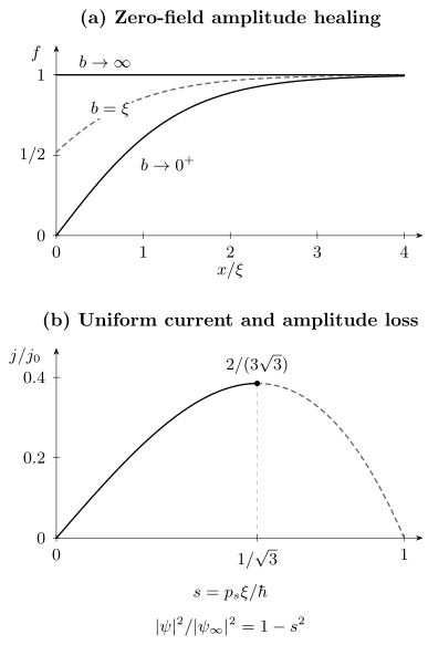
Two predictions that require a variable amplitude. Above: the zero-field surface profile for strong suppression, finite $b=\xi$ and a non-pair-breaking surface. Below: $j/j_0=s(1-s^2)$ has its maximum before the uniform amplitude vanishes. The descending branch is a stationary uniform solution, not an assertion of stability under arbitrary circuit conditions.

Near-transition predictions and their limits

For $\alpha\propto T-T_c$ and smooth $\beta,m^\ast$, the mean-field results are:

Quantity	Leading behavior below $T_c$
$\lvert\psi_\infty\rvert$	$(T_c-T)^{1/2}$
condensation-energy magnitude	$(T_c-T)^2$
$B_c$ and orbital $B_{c2}$	$T_c-T$
$\xi$ and $\lambda$	$(T_c-T)^{-1/2}$
$j_d$	$(T_c-T)^{3/2}$
$\kappa$	constant to leading order

Gor’kov’s microscopic derivation connects this expansion to weak-coupling BCS theory near $T_c$. It does not make coefficients universal or justify extrapolating every relation to low temperature. Anisotropic gradients require a mass tensor; several order parameters permit distinct healing lengths and relative-phase couplings. Unconventional Superconductivity explains how crystal symmetry constrains those fields.

Minimization is a mean-field description. Thermal fluctuations instead sample configurations with weight $e^{-F/(k_{\mathrm B}T)}$, with a cutoff, gauge treatment and boundary conditions. The Ginzburg criterion estimates when neglecting them fails. The static energy also does not specify time evolution: kinetic coefficients, conservation laws, dissipation and noise are additional physical input. A static GL fit alone cannot establish a vortex relaxation time or a nonequilibrium response.

Exercises

1. A finite extrapolation length

For a zero-field half-space with outward normal $-\hat{\mathbf x}$ and $b>0$, find the surface amplitude $f_0=f(0)$. Evaluate it at $b=\xi$ and identify the limits of weak and strong suppression.

Solution

The shifted tanh solution gives $f'(0)=(1-f_0^2)/(\sqrt2\xi)$. The boundary condition is $f'(0)=f_0/b$, so

$$\begin{aligned} u(1-f_0^2)&=\sqrt2 f_0,\qquad u=b/\xi,\\ f_0&=\frac{\sqrt2u}{\sqrt{1+2u^2}+1}. \end{aligned}$$

At $u=1$, $f_0\simeq0.5176$. As $u\to0^+$, $f_0\to0$; as $u\to\infty$, $f_0\to1$. The shift is $x_0=\sqrt2\xi\operatorname{artanh}f_0$. A positive surface energy suppresses the amplitude, confirming the outward-normal sign.

2. Three critical scales at one temperature

At a temperature within the GL regime, a hypothetical isotropic sample has $\lambda=200\,\mathrm{nm}$ and $\xi=20\,\mathrm{nm}$. Estimate $B_c$, $B_{c2}$ and $B_{c1}$, taking $c_{\rm core}=0.5$ only as an illustrative large-$\kappa$ approximation. Does a resistive onset determine all three?

Solution

The ratio is $\kappa=10$, giving

$$\begin{aligned} B_c&\simeq0.0582\,\mathrm T,\\ B_{c2}&\simeq0.823\,\mathrm T,\\ B_{c1}&\simeq0.0115\,\mathrm T. \end{aligned}$$

They satisfy $B_{c2}/B_c=\sqrt2\kappa$. The lower-field estimate is less precise because it uses a core approximation. A resistive onset alone cannot distinguish vortex motion, inhomogeneous transition paths and bulk thermodynamic loss of superconductivity. Independent magnetic and thermodynamic measurements are needed.

3. Derive the depairing maximum

Starting from the uniform free-energy density at fixed $p_s$, minimize over amplitude and then maximize the current. Explain why setting $|\psi|=0$ does not give the maximum current.

Solution

The quadratic coefficient becomes $\alpha+p_s^2/(2m^\ast)$. Minimization gives $|\psi|^2/|\psi_\infty|^2=1-s^2$ for $0\le s<1$. Hence

$$\frac{d(j/j_0)}{ds}=1-3s^2=0$$

at $s=1/\sqrt3$, with $j_d/j_0=2/(3\sqrt3)$. At $s=1$ the amplitude and current both vanish. The current maximum comes from competing increases in momentum and decreases in stiffness, not from complete destruction of the amplitude. With $j_0=\sqrt2B_c/(\mu_0\lambda)$, the stated dimensional formula follows.

4. Surface nucleation above the bulk transition

Suppose a phenomenological surface energy instead has $b<0$. Linearize the zero-field GL equation for $T>T_c$ in $x>0$. Can a decaying surface solution nucleate above the bulk $T_c$? State the model’s limitation.

Solution

Here $\alpha>0$. With $K=\hbar^2/(2m^\ast)$, the equation is $-K\psi''+\alpha\psi=0$. The decaying solution is $\psi\propto e^{-x\sqrt{\alpha/K}}$. The same outward-normal boundary condition gives $\psi'(0)=\psi(0)/b$, requiring

$$\begin{aligned} \alpha&=\frac{K}{b^2},\\ T_{\rm surf}-T_c&=\frac{K}{\alpha_0 b^2}>0. \end{aligned}$$

A surface that favors order can therefore nucleate it while the bulk remains normal. The quartic term stabilizes the finite amplitude below this onset. The prediction requires a physically justified surface coefficient and a shift small enough for the local near-$T_c$ expansion to apply; it is not a claim that an arbitrary surface enhances superconductivity.

References

• A. A. Abrikosov, “Nobel Lecture: Type-II superconductors and the vortex lattice,” Reviews of Modern Physics 76, 975–979 (2004), doi:10.1103/RevModPhys.76.975.
• P. G. de Gennes, Superconductivity of Metals and Alloys, W. A. Benjamin (1966).
• V. L. Ginzburg and L. D. Landau, “On the theory of superconductivity,” Zhurnal Eksperimental’noi i Teoreticheskoi Fiziki 20, 1064–1082 (1950); English translation in Collected Papers of L. D. Landau, 546–568 (1965), doi:10.1016/B978-0-08-010586-4.50078-X.
• L. P. Gor’kov, “Microscopic derivation of the Ginzburg–Landau equations in the theory of superconductivity,” Soviet Physics JETP 9, 1364–1367 (1959), official JETP archive.
• P. Lipavský, K. Morawetz, J. Koláček, and T. J. Yang, “Ginzburg–Landau theory of superconducting surfaces under the influence of electric fields,” Physical Review B 73, 052505 (2006), doi:10.1103/PhysRevB.73.052505.
• M. Tinkham, Introduction to Superconductivity, 2nd ed., Dover (2004).