BCS Theory

BCS theory relates coherent fermion pairing to excitation spectra, thermodynamics and electromagnetic stiffness. For matched time-reversed states at a Fermi surface with a finite density of states, an attractive Cooper channel produces a logarithmic instability and an exponentially small pairing scale. The elementary isotropic weak-coupling model then predicts quantitative ratios that can be tested across several measurements.

These ratios are benchmarks, not definitions of superconductivity. A paired mean-field structure can remain useful when anisotropy, several bands or retarded interactions change its simplest numbers. The full variational and operator derivation is developed in BCS Mean-Field Theory; this page connects its results to material observables.

Required background. The many-body Fermi Surface explains the low-energy shell; Density of States supplies state counting; Creation and Annihilation Operators supplies fermionic algebra; the Grand-Canonical Ensemble explains chemical potential.

Time-reversed pairs and the weak-coupling model

Take a clean, translationally invariant, single-band, spin-singlet $s$-wave model, with $\xi_{\mathbf k}=\varepsilon_{\mathbf k}-\mu$ and $\xi_{-\mathbf k}=\xi_{\mathbf k}$. Let $N(0)$ be the normal density of states per spin and per unit volume. An attractive contact matrix element $g>0$ has units of energy times volume, so the dimensionless coupling is $\lambda_{\rm BCS}=N(0)g$.

For volume $\mathcal V$, define $b_{\mathbf k}^\dagger=c_{\mathbf k\uparrow}^\dagger c_{-\mathbf k\downarrow}^\dagger$. The reduced model is

$$\begin{aligned} K&=\sum_{\mathbf k\sigma}\xi_{\mathbf k}c_{\mathbf k\sigma}^\dagger c_{\mathbf k\sigma} -\frac g{\mathcal V}B^\dagger B,\\ B&=\sum_{\mathbf k\ \mathrm{in\ shell}}b_{\mathbf k}. \end{aligned}$$

The shell has energy cutoff $\Omega_c$, schematically $\hbar\omega_D$ for phonon pairing. The weak-coupling formulas assume $\lambda_{\rm BCS}\ll1$, a nearly constant density of states over the shell and $\Omega_c\ll E_F$. Keep the microscopic shell fixed when differentiating thermodynamic quantities; moving a sharp cutoff with $\mu$ changes the effective Hamiltonian.

The pair susceptibility contains $N(0)\int d\xi/\xi$. With temperature as its infrared cutoff, it grows logarithmically as $T\to0$. In the ideal thermodynamic, matched-Fermi-surface problem, any attractive eigenvalue can therefore cause pairing. Finite level spacing, pair breaking, Fermi-surface mismatch or a vanishing density of states can cut off or remove this conclusion. The Cooper instability is more specific than the claim that two isolated particles bind.

Phonons provide one microscopic source of retarded attraction: an electron couples to a lattice deformation that subsequently affects another electron. The reduced model replaces the frequency-dependent interaction by a constant attractive shell. A spectral fit to that simplified model does not, by itself, establish that phonons supplied the attraction.

Pair field and quasiparticle spectrum

The pair potential is $\Delta=(g/\mathcal V)\langle B\rangle$. The exact quartic Hamiltonian conserves particle number. Its mean-field representative permits a coherent superposition of empty and doubly occupied time-reversed orbitals. Fixed-number projection is available when finite-system parity or number fluctuations matter; the exact reduced model treats finite levels without the anomalous mean-field replacement.

For the spinor $(c_{\mathbf k\uparrow},c_{-\mathbf k\downarrow}^\dagger)^{\mathsf T}$ and this definition of $\Delta$,

$$\mathcal H_{\mathbf k}= \begin{pmatrix}\xi_{\mathbf k}&-\Delta\\-\Delta^\ast&-\xi_{\mathbf k}\end{pmatrix}.$$

Its eigenvalues are $\pm E_{\mathbf k}$, with $E_{\mathbf k}=\sqrt{\xi_{\mathbf k}^2+|\Delta|^2}$. Negative Nambu energies are particle–hole partners, not an extra species of negative-energy particles. For real positive $\Delta$, the positive eigenvector can be chosen as $(u,-v)$, where

$$\begin{aligned} u^2&=\frac12(1+\xi/E),\\ v^2&=\frac12(1-\xi/E),\\ uv&=\frac{\Delta}{2E}. \end{aligned}$$

The minus sign in the eigenvector belongs with the minus signs in this Nambu matrix. The positive pair amplitude in the variational state uses $u+v b^\dagger$ in the same convention.

The mean-field charge expectation of an added quasiparticle is $-e(u^2-v^2)=-e\xi/E$. It changes continuously from electron-like to hole-like and vanishes at $\xi=0$. It is not a separately conserved charge eigenvalue: the excitation can exchange charge with the condensate.

Gap scale and transition benchmarks

For a real gap magnitude, self-consistency reduces to

$$\begin{aligned} \lambda_{\rm BCS}^{-1} &=\int_0^{\Omega_c}\frac{d\xi}{E(\xi)} \tanh\frac{E(\xi)}{2k_BT},\\ E(\xi)&=\sqrt{\xi^2+\Delta^2(T)}. \end{aligned}$$

The pair kernel originally contains $1/(2E)$ and a shell on both sides of the Fermi level. Symmetry combines those two halves, leaving the per-spin $N(0)$ with no extra factor of two. At fixed density, a number equation must also determine $\mu$; this is especially important for narrow bands and the BCS–BEC crossover.

At zero temperature, the integral is $\operatorname{arsinh}(\Omega_c/\Delta_0)$, giving

$$\begin{aligned} \Delta_0&=\frac{\Omega_c}{\sinh(1/\lambda_{\rm BCS})},\\ &\simeq2\Omega_c e^{-1/\lambda_{\rm BCS}}. \end{aligned}$$

Linearizing at the mean-field transition gives, in the same weak-coupling limit,

$$\begin{aligned} k_BT_c&\simeq\frac{2e^{\gamma_E}}\pi \Omega_c e^{-1/\lambda_{\rm BCS}},\\ \frac{2\Delta_0}{k_BT_c}&\longrightarrow \frac{2\pi}{e^{\gamma_E}}\simeq3.528. \end{aligned}$$

Here $\gamma_E$ is Euler’s constant. The ratio is asymptotic: finite cutoff-to-gap corrections change it. Close to the mean-field $T_c$,

$$\Delta(T)\simeq3.06\,k_BT_c\sqrt{1-T/T_c}.$$

In a phase-fluctuation-dominated material, this pairing scale need not be the actual superconducting transition. Two-dimensional vortex physics or granular connectivity can suppress global coherence.

Pair correlations and material length scales

The clean weak-coupling Pippard–BCS length is $\xi_0=\hbar v_F/(\pi\Delta_0)$. For a parabolic band,

$$k_F\xi_0=\frac{2E_F}{\pi\Delta_0}\gg1.$$

Thus weak-coupling pair correlations overlap strongly in space. This scale is not the unique root-mean-square size of every possible pair wavefunction; definitions based on anomalous correlations, two-particle states and response kernels can differ by numerical factors.

Length	Physical use
$\xi_0=\hbar v_F/(\pi\Delta_0)$	clean weak-coupling correlation and nonlocal-response scale
$\xi_{\rm GL}(T)$	amplitude and nucleation scale near a continuous transition
$\sqrt{\Phi_0/(2\pi B_{c2})}$	field-inferred length when the orbital model applies
$\sqrt{\hbar D/\Delta}$	diffusive coherence scale, with convention-dependent factors

For a hypothetical sample with $T_c=10.0\,\mathrm K$, $\Delta_0=1.90\,\mathrm{meV}$ and $v_F=3.0\times10^5\,\mathrm{m\,s^{-1}}$, the ratio is $4.41$ and the clean estimate is $\xi_0\simeq33\,\mathrm{nm}$. The larger-than-BCS ratio motivates tests of strong coupling, anisotropy, several gaps and fit broadening; it identifies none of them uniquely. The estimated length should not be relabeled a GL healing length without an appropriate relation.

Thermodynamic tests

To leading order in weak coupling, the zero-temperature condensation energy per volume and normal electronic heat-capacity coefficient are

$$\begin{aligned} f_s-f_n&\simeq-\tfrac12N(0)\Delta_0^2,\\ \gamma_n&=\frac{2\pi^2}{3}k_B^2N(0),\\ C_n&=\gamma_nT. \end{aligned}$$

The factor two in $\gamma_n$ counts spin. The resulting ratio $(f_n-f_s)/(\gamma_nT_c^2)\simeq0.236$ connects an integrated thermodynamic measurement to a spectroscopic gap. The condensation energy also equals $B_c^2/(2\mu_0)$ in the ideal bulk comparison; a resistive onset or first vortex-entry field is a different quantity.

The quasiparticle entropy per volume is

$$\begin{aligned} s_s&=-\frac{2k_B}{\mathcal V}\sum_{\mathbf k} h(f_{\mathbf k}),\\ h(f)&=f\ln f+(1-f)\ln(1-f),\\ f_{\mathbf k}&=[e^{E_{\mathbf k}/(k_BT)}+1]^{-1}. \end{aligned}$$

Differentiating $C_s=T\,ds_s/dT$ must include the self-consistent temperature dependence of $\Delta$. This gives

$$\frac{\Delta C}{\gamma_nT_c} =\frac{12}{7\zeta(3)}\simeq1.426$$

in the isotropic weak-coupling limit. A full gap gives an activated low-temperature electronic heat capacity; nodes can give powers. Strong coupling, gap anisotropy, nonsuperconducting volume and phonon subtraction all affect a measured jump. Heat Capacity and Thermodynamics explains the entropy and background checks.

Tunneling spectra and spectral weight

Tunneling probes the electron spectral density, not an unweighted count of all positive-energy quasiparticle modes. In the particle–hole-symmetric constant-DOS model, the electron spectrum per spin is

$$N_s(E)=N(0)\operatorname{Re} \frac{|E|}{\sqrt{E^2-\Delta^2}}.$$

Electron and hole coherence weights combine the two roots in $\xi$. Counting positive excitation energies without those weights instead gives a different normalization. The ideal electron spectrum has no weight for $|E|<\Delta$ and integrable edge singularities proportional to $(|E|-\Delta)^{-1/2}$.

For phenomenological Dynes broadening, put $z=E+i\Gamma$ with $\Gamma>0$:

$$\frac{N_\Gamma(E)}{N(0)} =\operatorname{Re}\frac{z}{\sqrt{z-\Delta}\sqrt{z+\Delta}}.$$

The two individual square roots use their principal branches, so their product is the retarded root analytic in the upper half-plane and asymptotic to $z$. Taking the principal square root directly of $z^2-\Delta^2$ gives the wrong sign at negative energy. The correct spectrum is positive and even. A fit parameter $\Gamma$ is not automatically a microscopic scattering rate; inhomogeneity, resolution, anisotropy and pair breaking can produce similar rounding. Herman and Hlubina (2016) give one specified microscopic realization.

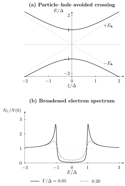
The upper panel shows $E/\Delta=\pm\sqrt{1+(\xi/\Delta)^2}$ and the normal crossing. The lower panel uses the stated retarded Dynes root for $\Gamma/\Delta=0.05$ and $0.20$. Increasing broadening rounds the coherence peaks and fills the hard gap; these curves are electron spectra before thermal tunneling convolution.

For a normal tip with approximately constant density of states and an energy-independent tunneling matrix element,

$$\frac{dI}{dV}\propto\int dE\,N_s(E) \left[-\frac{\partial f(E-eV)}{\partial E}\right].$$

Only at sufficiently low temperature and resolution width does this closely trace $N_s(eV)$. Thermal convolution can produce nonzero zero-bias conductance even when the underlying spectrum has a hard gap. A superconducting tip supplies another gapped spectrum. Tunneling Spectroscopy develops these measurement details.

Response depends on the probe

A density of states alone does not determine a response. Current, spin and density vertices carry different coherence factors, including relative gap phases. Consequently:

• NMR relaxation can show a Hebel–Slichter enhancement, but fields and inelastic or pair-breaking processes may remove it. A simple lifetime broadening is not equivalent to every kind of nonmagnetic disorder.
• Penetration depth is activated in a fully gapped local clean benchmark, with directional and nonlocal qualifications discussed in London Theory.
• Optical pair creation depends on momentum relaxation and vertex physics. A gap in the electron spectrum does not ensure finite uniform-current absorption immediately above $2\Delta$ in an ideal clean continuum.

For the pair phase convention $\Delta\propto\langle cc\rangle$, the local electromagnetic limit is

$$\mathbf j_s=-\frac{1}{\mu_0\lambda^2} \left(\mathbf A+\frac{\hbar}{2e}\boldsymbol\nabla\theta\right).$$

The combination is gauge invariant because $\theta\mapsto\theta-2e\chi/\hbar$. Its coefficient requires the full gauge-consistent response, including diamagnetic and paramagnetic terms. A pairing amplitude alone does not prove a nonzero Meissner stiffness in every geometry or model.

Retardation, isotope shifts and extensions

If only ionic mass changes, $\omega_D\propto M^{-1/2}$ and a mass-independent coupling give $\alpha_{\rm iso}=-d\ln T_c/d\ln M=1/2$. Coulomb retardation, anharmonicity, several modes and structural changes can alter this exponent without excluding phonons.

Migdal–Eliashberg theory retains frequency-dependent gap and electron self-energies. Its electron–phonon spectrum $\alpha^2F(\omega)$ determines

$$\lambda_{\rm ep}=2\int_0^\infty\frac{\alpha^2F(\omega)}\omega\,d\omega.$$

This coupling is not simply the reduced-model $\lambda_{\rm BCS}$. The Coulomb pseudopotential is often approximated by

$$\mu^\ast=\frac{\mu_C}{1+\mu_C\ln(E_{\rm el}/\Omega_{\rm ph})},$$

where $\mu_C$ is a dimensionless screened repulsion, not chemical potential. McMillan–Allen–Dynes estimates further use a logarithmic phonon frequency and spectral-shape corrections; their numerical interpolation is meaningful only with a justified phonon spectrum and controlled neglect of vertex corrections (Allen and Dynes, 1975; Carbotte, 1990).

Anisotropic or sign-changing gaps require momentum-dependent pairing. Multiple bands require coupled gap equations and different experimental weights. Anderson’s theorem protects the ideal isotropic $s$-wave transition against a limited class of nonmagnetic disorder; strong inhomogeneity, localization and pair breaking fall outside its assumptions. Low density requires the number equation and possibly BCS–BEC crossover physics. Unconventional Superconductivity explains how symmetry and several probes constrain these alternatives.

Exercises

1. Check the finite-cutoff correction

For $\lambda_{\rm BCS}=0.20$ and $0.50$, compare the exact zero-temperature sharp-shell gap with $2\Omega_c e^{-1/\lambda_{\rm BCS}}$. Why is the ratio $3.528$ also only asymptotic?

Solution

The exact-to-asymptotic gap ratio is

$$\frac{1}{1-e^{-2/\lambda_{\rm BCS}}}.$$

It is approximately $1.000045$ for $0.20$ and $1.01866$ for $0.50$. The transition-temperature integral also retains a finite upper cutoff. Both approximations must be checked before treating their quotient as a universal number. The full numerical ratios for this model are about $3.52791$ and $3.59214$, respectively; the latter is a finite-cutoff benchmark, not a controlled weak-coupling material prediction.

2. Follow a state through the gap

For real positive $\Delta$, verify that the positive eigenvector of the displayed Nambu matrix is $(u,-v)$, and interpret its charge at $\xi/\Delta=0$ and $\pm3$.

Solution

The first row requires $(E-\xi)u=\Delta v$, consistent with $u^2=(1+\xi/E)/2$ and positive $uv=\Delta/(2E)$. The charge is $-e\xi/E$. It is zero at $\xi=0$, and equals $\mp3e/\sqrt{10}\simeq\mp0.949e$ at $\xi/\Delta=\pm3$. The zero value reflects equal particle and hole weights; it does not make quasiparticle number into a conserved neutral-particle charge.

3. Gap filling versus thermal conductance

Find the Dynes spectral density at $E=0$. For an ideal hard gap, can finite-temperature tunneling nevertheless give a nonzero zero-bias conductance?

Solution

The retarded root at $z=i\Gamma$ is $i\sqrt{\Gamma^2+\Delta^2}$, giving

$$\frac{N_\Gamma(0)}{N(0)} =\frac{\Gamma}{\sqrt{\Gamma^2+\Delta^2}}.$$

For a hard gap with $\Gamma=0$, the spectrum vanishes below $\Delta$, but the finite-temperature derivative of the Fermi function samples states above both gap edges. In the low-temperature limit, using $E=\Delta\cosh u$ gives

$$\frac{G(0,T)}{G_n} \simeq\sqrt{\frac{2\pi\Delta}{k_BT}} \,e^{-\Delta/(k_BT)}.$$

It is exponentially small but nonzero. Spectral gap filling and thermal smearing are therefore distinct effects that must both enter a conductance fit.

4. Compare thermodynamic measurements

For $T_c=8.0\,\mathrm K$ and molar $\gamma_n=25\,\mathrm{mJ\,mol^{-1}K^{-2}}$, estimate the weak-coupling heat-capacity jump and zero-temperature condensation energy per mole.

Solution

$$\begin{aligned} \Delta C&\simeq1.426\gamma_nT_c,\\ &\simeq285\,\mathrm{mJ\,mol^{-1}K^{-1}},\\ F_n-F_s&\simeq0.236\gamma_nT_c^2,\\ &\simeq0.378\,\mathrm{J\,mol^{-1}}. \end{aligned}$$

The same normal reference and superconducting fraction must be used in both comparisons. Agreement constrains integrated thermodynamics, but does not determine gap phase or pairing mechanism.

5. A mass-dependent interaction

Let $T_c=CM^{-1/2}e^{-1/\lambda(M)}$ and $\beta_M=d\ln\lambda/d\ln M$. Find the isotope exponent.

Solution

Differentiating $\ln T_c=\ln C-\tfrac12\ln M-1/\lambda$ gives

$$\alpha_{\rm iso}=\frac12-\frac{\beta_M}{\lambda}.$$

Thus the value $1/2$ requires mass-independent coupling as well as the assumed phonon-frequency scaling. An anomalous exponent alone does not identify the pairing interaction.

References

• P. B. Allen and R. C. Dynes, “Transition Temperature of Strong-Coupled Superconductors Reanalyzed,” Physical Review B 12, 905–922 (1975), doi:10.1103/PhysRevB.12.905.
• J. Bardeen, L. N. Cooper, and J. R. Schrieffer, “Theory of Superconductivity,” Physical Review 108, 1175–1204 (1957), doi:10.1103/PhysRev.108.1175.
• J. P. Carbotte, “Properties of Boson-Exchange Superconductors,” Reviews of Modern Physics 62, 1027–1157 (1990), doi:10.1103/RevModPhys.62.1027.
• L. N. Cooper, “Bound Electron Pairs in a Degenerate Fermi Gas,” Physical Review 104, 1189–1190 (1956), doi:10.1103/PhysRev.104.1189.
• F. Herman and R. Hlubina, “Microscopic interpretation of the Dynes formula for the tunneling density of states,” Physical Review B 94, 144508 (2016), doi:10.1103/PhysRevB.94.144508. The retarded square-root branch and a specified microscopic broadening model.
• P. Morel and P. W. Anderson, “Calculation of the Superconducting State Parameters with Retarded Electron-Phonon Interaction,” Physical Review 125, 1263–1271 (1962), doi:10.1103/PhysRev.125.1263.
• M. Tinkham, Introduction to Superconductivity, 2nd ed., Dover (2004).