Heat Capacity and Thermodynamics

Heat capacity measures the heat required to raise a sample’s temperature under specified constraints. Its temperature dependence tells us which excitations become thermally accessible: acoustic phonons, electrons near a Fermi surface, magnetic levels, or collective modes. Integrating $C/T$ gives an entropy difference and helps test whether a proposed set of excitations can explain the measurement.

The thermometer usually measures a small platform attached to the sample. The sample must exchange heat with that platform quickly enough to follow the measurement. We first connect the recorded temperature to heat capacity, then interpret low-temperature fits and transition anomalies. Calorimetry counts excitations throughout the thermally coupled sample; identifying them usually also requires spectroscopy, scattering, or magnetic response.

Required background. How Quantum Matter Is Measured supplies calibration, background subtraction and uncertainty checks. Thermodynamic Potentials supplies the natural variables and fixed-control derivatives defining heat capacities. Entropy supplies the equilibrium meaning of thermal entropy and its distinction from other state-entropy measures.

Heat capacity and the held variables

Heating changes both the internal energy and, potentially, the work done by the sample. This is why a freely expanding crystal and a clamped crystal need not have the same heat capacity.

For a reversible path with generalized controls $X$ held fixed,

$$C_X = T \left( \frac{\partial S}{\partial T} \right)_X = \left( \frac{\delta Q_{\mathrm{rev}}}{dT} \right)_X.$$

For a closed sample with only pressure–volume work, at constant volume,

$$C_V = \left( \frac{\partial U}{\partial T} \right)_{V,N,\ldots},$$

whereas at constant pressure,

$$C_p = \left( \frac{\partial H}{\partial T} \right)_{p,N,\ldots}.$$

Low-pressure calorimetry on a freely expanding solid usually approximates $C_p$. Many microscopic models calculate $C_V$. For an isotropic equilibrium solid,

$$C_p-C_V = \frac{ TV\alpha_V^2 }{ \kappa_T } = TVB_T\alpha_V^2,$$

where $\alpha_V$ is the volume expansion coefficient, $\kappa_T$ the isothermal compressibility, and $B_T=1/\kappa_T$. The expansion coefficient here is volumetric, not the linear coefficient; for isotropic expansion $\alpha_V=3\alpha_L$. The difference is often small at cryogenic temperatures, but it can matter near structural transitions and soft modes. Barron and White explain this conversion and its low-temperature limits.

Specify magnetic field, pressure or strain, composition, and particle number as appropriate. With additional work terms, use the potential appropriate to those controls rather than transferring the formulas for $U$ or $H$ unchanged. A field-swept or pressure-swept calorimetric protocol is not automatically the same derivative as a temperature sweep at fixed field or pressure.

Total, specific, and molar heat capacity

Use distinct notation and units for:

• total heat capacity $C$ in $\mathrm{J\,K^{-1}}$;
• mass-specific heat capacity $c=C/m$ in $\mathrm{J\,kg^{-1}\,K^{-1}}$;
• molar heat capacity $C_m=C/n_{\mathrm{mol}}$ in $\mathrm{J\,mol^{-1}\,K^{-1}}$;
• volumetric heat capacity $C/V$ in $\mathrm{J\,m^{-3}\,K^{-1}}$.

In materials papers, “specific heat” often means molar heat capacity. That usage is conventional but ambiguous. State whether one mole means formula units, atoms, magnetic ions, or another counted object. The distinction enters every comparison with $R\ln g$, $3nR$, a Sommerfeld coefficient, or a phase fraction.

From heater power to heat capacity

Relaxation calorimetry

Relaxation calorimetry, developed for small samples by Bachmann and collaborators, mounts a sample on a small platform containing a heater and thermometer. A weak thermal link of conductance $K$ connects the platform to a bath at temperature $T_b$. In the one-node, small-excursion model,

$$\begin{aligned} C_{\mathrm{tot}}\frac{d\delta T}{dt}&=P(t)-K\delta T,\\ \delta T&=T-T_b. \end{aligned}$$

After the heater is switched off,

$$\delta T(t) = \delta T_0e^{-t/\tau}, \qquad \tau = \frac{C_{\mathrm{tot}}}{K}.$$

The sample heat capacity is then inferred from

$$C_{\mathrm{samp}} = C_{\mathrm{tot}} -C_{\mathrm{add}},$$

where $C_{\mathrm{add}}$ includes the platform, thermometer, heater, leads, grease, and any substrate or capsule that participates thermally.

Stewart reviews the practical limits of this measurement. This single exponential is valid only when the sample and platform share one temperature, $C$ and $K$ are effectively constant across the pulse, the bath remains fixed, radiative and parasitic heating are negligible, and the transition does not release latent heat during the decay. A good fit residual is necessary but not sufficient: several thermal modes can masquerade as one over a short time window.

Internal thermalization and the two-node model

Poor sample contact or low internal thermal diffusivity creates a second time scale. A minimal two-node model uses a sample temperature $T_s$, platform temperature $T_a$, sample–platform conductance $K_s$, and bath conductance $K_b$:

$$\begin{aligned} C_s\dot T_s&=-K_s(T_s-T_a), \\ C_a\dot T_a&=P(t)-K_b(T_a-T_b) +K_s(T_s-T_a). \end{aligned}$$

Adding these two equations gives $C_s\dot T_s+C_a\dot T_a=P-K_b(T_a-T_b)$: internal heat exchange cancels, as energy conservation requires. Brando gives the corresponding two-temperature relaxation analysis. The platform response is generally a sum of two exponentials. The fast internal mode tests whether the sample equilibrates with the thermometer; the slow external mode describes cooling to the bath. If the time scales are not resolved or the sample has distributed thermal diffusion, a lumped two-node fit can still bias $C_s$.

Thermal grease improves contact but adds heat capacity. A tiny crystal with heat capacity much smaller than the addenda is obtained as a difference between comparable numbers, amplifying mass, fit, and background uncertainty. Measure the empty platform with the same field, temperature, wiring, and grease preparation. For the subtraction $C_s=C_{\mathrm{tot}}-C_a$, the propagated variance is

$$u^2(C_s)=u^2(C_{\mathrm{tot}})+u^2(C_a) -2\operatorname{Cov}(C_{\mathrm{tot}},C_a).$$

Shared calibration errors may correlate the two measurements. Treating every error as independent can therefore overestimate or underestimate the uncertainty; the JCGM guide explains this propagation.

Heat pulses and periodic heating

A nearly adiabatic pulse supplies heat $Q=\int P(t)\,dt$. For a single equilibrium phase, after correcting heat loss to the bath,

$$Q\simeq\int_{T_i}^{T_f}C_X(T)\,dT.$$

A small pulse gives $C_X\simeq Q/\Delta T$; a larger pulse gives an interval average. If a first-order transition is crossed, include its latent heat separately. A temperature plateau can absorb energy without a corresponding temperature rise.

In ac calorimetry, introduced by Sullivan and Seidel, periodic heating produces a small temperature oscillation. Let $P(t)=\bar P+\operatorname{Re}[P_\omega e^{i\omega t}]$ and $T(t)=\bar T+\operatorname{Re}[T_\omega e^{i\omega t}]$. Linearizing about the heated mean temperature gives

$$\begin{aligned} T_\omega&=\frac{P_\omega}{K+i\omega C},\\ |T_\omega|&=\frac{|P_\omega|}{\sqrt{K^2+(\omega C)^2}},\\ \phi&=\tan^{-1}(\omega C/K). \end{aligned}$$

Here $\phi$ is the positive lag of temperature behind power. The angular frequency belongs to the heating power: a current $I_0\cos\Omega t$ through a constant resistance produces a dc term and an oscillating power at $\omega=2\Omega$, each of magnitude $I_0^2R/2$.

When $\omega C\gg K$, heat leakage per cycle is small and

$$C\simeq\frac{|P_\omega|}{\omega|T_\omega|}.$$

Increasing frequency indefinitely does not improve the measurement: eventually the sample cannot follow the platform. For the preceding two-node model, solve the sample equation first, with $\tau_s=C_s/K_s$:

$$\begin{aligned} T_{s,\omega}&=\frac{T_{a,\omega}}{1+i\omega\tau_s},\\ Y(\omega)\equiv\frac{P_\omega}{T_{a,\omega}} &=K_b+i\omega C_a +\frac{i\omega C_s}{1+i\omega\tau_s}. \end{aligned}$$

This is the thermal admittance: power divided by the measured temperature oscillation. Its out-of-phase part gives

$$C_{\mathrm{phase}}\equiv\frac{\operatorname{Im}Y}{\omega} =C_a+\frac{C_s}{1+(\omega\tau_s)^2}.$$

At low frequency it includes the sample; at high frequency it tends to the platform heat capacity alone. The amplitude estimate $C_{\mathrm{amp}}=|Y|/\omega$ also includes the in-phase heat flow. To approximate the full equilibrium heat capacity with the amplitude method, seek an interval satisfying

$$\frac{K_b}{C_a+C_s}\ll\omega\ll\frac{K_s}{C_s}.$$

Other thermometer, heater, and internal diffusion times must also be short compared with $1/\omega$. A frequency scan tests whether such an interval exists. An intrinsic slow degree of freedom can also produce dynamic heat capacity, but a frequency dependence caused by poor contact should not be assigned to new sample physics.

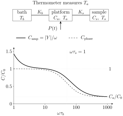
The two-node model with $C_a=0.2C_0$, $C_s=0.8C_0$, and $\tau_s=0.02\tau_b$, where $C_0=C_a+C_s$ and $\tau_b=C_0/K_b$. The amplitude estimate is too large at low frequency because of bath leakage. At intermediate frequency both estimates are near $C_0$. At high frequency the sample decouples, and both approach $C_a$. These are calculated responses of a calorimeter with constant heat capacities, not a material phase transition.

Thermometer and protocol controls

The thermometer must be calibrated in temperature and field on the mounted platform. Self-heating, magnetoresistance, field-sweep eddy currents, wiring heat leaks, bath drift, and finite controller bandwidth can all create false anomalies. The heater power is $P=I^2R$ only after current, heater resistance, waveform, and lead configuration are known at the measurement condition.

Repeat measurements with different pulse sizes or frequencies, compare warming and cooling, and inspect the raw curves near an anomaly. A reference material or a second mounting tests whether the feature belongs to the sample or to its thermal contact.

Separating electronic, lattice, and magnetic contributions

Write the measured molar heat capacity schematically as

$$C_m=C_{\mathrm{el}}+C_{\mathrm{ph}}+C_{\mathrm{mag}} +C_{\mathrm{nuc}}+C_{\mathrm{def}}+C_{\mathrm{tr}}+\cdots.$$

This decomposition organizes analysis, but it is not exact when sectors are strongly coupled. Magnetoelastic modes, electron–phonon renormalization, hybridization, and collective order can redistribute entropy between nominal components. A background should therefore be described as a model for the non-target terms, not as the uniquely known lattice or electronic heat capacity.

Useful background strategies include:

• a low-temperature expansion over a justified asymptotic window;
• a field-suppressed normal state, if field does not substantially alter other terms;
• an isostructural nonmagnetic analog with mass and phonon corrections;
• a first-principles or measured phonon density of states;
• a global fit constrained simultaneously by several fields, compositions, or pressure values.

Each strategy has failure modes. A nonmagnetic analog can have different force constants or electronic structure. A high field can add Zeeman and nuclear terms. A polynomial can absorb the anomaly being sought.

Electronic heat capacity

Sommerfeld coefficient

For a Fermi liquid with a finite quasiparticle density of states, at temperatures small compared with the relevant Fermi scale,

$$C_{\mathrm{el}} = \gamma T+o(T),$$

with

$$\gamma = \frac{\pi^2}{3} k_{\mathrm B}^2 D^*(E_{\mathrm F}).$$

The notation $o(T)$ means that the correction divided by $T$ tends to zero. Here $D^*(E_{\mathrm F})$ is the quasiparticle density of states summed over bands and spin, in the same amount convention as $\gamma$. It is the thermodynamic density of states, not necessarily the electron spectral weight measured by tunneling. Subleading terms need not be an analytic cubic power: interactions and dimensionality can introduce nonanalytic temperature dependence. The Sommerfeld Expansion derives the ideal-gas result. In a material, mass renormalization, band multiplicity, electron–phonon coupling, and correlations enter the measured coefficient.

In an ordinary three-dimensional metal whose leading phonon term is $\beta T^3$,

$$\frac{C_m}{T} = \gamma +\beta T^2 +\delta T^4 +\cdots.$$

A $C_m/T$ versus $T^2$ plot makes $\gamma$ the intercept and $\beta$ the initial slope only within the asymptotic regime. Curvature, superconductivity, magnetism, nuclear terms, Schottky tails, dimensional crossover, or a non-Fermi-liquid contribution invalidate a two-parameter straight-line fit.

What a large gamma means

A large $\gamma$ establishes a large low-energy entropy density relative to temperature. In a coherent Fermi liquid it corresponds to a large quasiparticle density of states and often a large effective mass. It does not alone prove a heavy-fermion ground state, identify which bands are heavy, or distinguish intrinsic quasiparticles from low-energy disorder, two-level systems, or unresolved magnetic contributions.

The Wilson ratio combines $\gamma$ with the spin susceptibility and can test a quasiparticle interpretation, but only after core diamagnetism, Van Vleck terms, $g$ factors, and amount conventions are aligned. Quantum oscillations, ARPES, transport, and magnetic response provide independent constraints.

Phonon heat capacity

Phonons derives the mode contribution to heat capacity. Debye–Einstein Models compares spectral approximations and their mode counts; here we use those results to interpret a measured coefficient.

Debye coefficient

For a three-dimensional crystal with gapless acoustic phonons and linear long-wavelength dispersion,

$$C_{\mathrm{ph}} = \beta T^3 +O(T^5).$$

When $C_m$ is per mole of formula units containing $n$ atoms,

$$\beta = \frac{ 12\pi^4 }{ 5 } \frac{ nR }{ \Theta_{\mathrm D}^3 },$$

so an effective low-temperature Debye temperature is

$$\Theta_{\mathrm D} = \left( \frac{ 12\pi^4nR }{ 5\beta } \right)^{1/3}.$$

This convention extends an effective acoustic spectrum to $3n$ modes per formula unit; it does not mean there are $3n$ acoustic branches. A primitive cell has three acoustic branches, while any additional branches are optical. This $\Theta_{\mathrm D}$ summarizes the acoustic density of states sampled in the fit window. It need not equal a Debye temperature inferred from elastic constants, diffraction, a full-temperature fit, or another convention.

The harmonic treatment in Ashcroft and Mermin gives the following high-temperature limit. At temperatures above all harmonic phonon scales, the lattice contribution approaches the Dulong–Petit limit $3nR$ per mole of formula units. Real measurements can deviate because optical modes are not yet saturated, thermal expansion converts $C_V$ to $C_p$, anharmonicity changes frequencies, electronic or magnetic terms persist, or a structural transition intervenes.

Beyond one cubic term

The $T^3$ law assumes three-dimensional linear acoustic branches and a sufficiently low temperature. Layered crystals can show crossovers rather than a pure two-dimensional power law because any finite interlayer coupling restores three-dimensional behavior at the longest wavelength. Soft optical modes, rattling modes, disorder, vacancies, and anharmonicity add non-Debye structure.

An Einstein-like optical contribution has the form

$$C_E = N_Ek_{\mathrm B} \left( \frac{\Theta_E}{T} \right)^2 \frac{ e^{\Theta_E/T} }{ \left( e^{\Theta_E/T}-1 \right)^2 },$$

where $N_E$ counts oscillator modes in the amount being reported. For $M_E$ modes per formula unit and a molar heat capacity, $N_Ek_{\mathrm B}=M_ER$. Fitting several Einstein temperatures is descriptive unless spectroscopy or a phonon calculation constrains the modes and weights. A broad phonon density of states should not be turned into a collection of physically named oscillators merely because the fit is excellent.

Phase-transition anomalies

What an anomaly establishes

Heat capacity is a second temperature derivative of a thermodynamic potential. It is therefore sensitive to bulk nonanalyticity even when a minority conductive path dominates transport or a surface probe sees only a reconstructed layer. A reproducible entropy-carrying anomaly shows thermodynamic participation, but its size is weighted by the amount of material contributing. A minority phase can also produce a peak; a calorimetric anomaly alone does not establish a unit phase fraction.

They are not self-labeling. A lambda-shaped peak can arise near a continuous magnetic, structural, charge-order, ferroelectric, or superconducting transition. A broad maximum can be a crossover, short-range order, a Schottky anomaly, a glassy distribution, or a strongly broadened transition. Identify the order parameter with a symmetry-sensitive measurement.

Continuous transitions

Near a continuous transition at $T_c$, define reduced temperature

$$t = \frac{T-T_c}{T_c}.$$

The singular contribution is often parameterized as

$$C_{\mathrm{sing}} = A_\pm \lvert t\rvert^{-\alpha},$$

with different amplitudes above and below $T_c$ plus analytic backgrounds and corrections to scaling. For $\alpha<0$, this singular term does not diverge; it often produces a finite cusp on top of the regular background. At $\alpha=0$, a logarithm can replace the power law, and the expression above is not a complete description. Fisher reviews these distinctions. Thus absence of an infinite peak does not exclude a continuous transition.

Real anomalies are rounded by finite resolution, sample inhomogeneity, strain, disorder, finite size, temperature gradients, and pulse averaging. Fitting a critical exponent requires a reduced-temperature window wide enough to resolve scaling but narrow enough to suppress regular backgrounds and crossover physics. The transition temperature, amplitudes, background, correction terms, and convolution width are correlated; they should not be fixed opportunistically.

First-order transitions and latent heat

At an ideal equilibrium first-order transition, the entropy jumps by $\Delta S$ and the latent heat is

$$L = T_t\Delta S.$$

Formally, a temperature scan contains

$$C_p(T) = C_{\mathrm{reg}}(T) +L\delta(T-T_t).$$

A finite experiment spreads that energy over time and temperature. A relaxation curve may pause, develop multiple slopes, or become history dependent, violating the single-exponential model. Lashley and collaborators show why a standard relaxation analysis can miss latent heat. Compare integrated heat, warming and cooling, sweep rate, and independently measured coexistence or symmetry change. Hysteresis alone does not prove equilibrium first order because thermal lag and slow kinetics can also produce it.

Superconducting transitions

For weak-coupling isotropic BCS theory (Bardeen, Cooper, and Schrieffer; see Johnston for a detailed thermodynamic treatment),

$$\frac{ \Delta C_{\mathrm{el}}(T_c) }{ \gamma_nT_c } \simeq 1.426.$$

This is a benchmark, not a universal criterion. Strong coupling, gap anisotropy, multiple bands, pair breaking, fluctuations, transition broadening, and incomplete superconducting volume all change the measured jump. A field-suppressed normal-state reference is useful only if the field does not introduce comparably important magnetic, nuclear, vortex, or normal-state changes.

At a continuous zero-field transition, the two phases have equal entropy at $T_c$. If their extrapolated zero-temperature entropies also agree, this becomes

$$\int_0^{T_c} \frac{ C_s(T)-C_n(T) }{ T } \,dT = 0.$$

Failure can expose an incorrect background, missing low-temperature extrapolation, transition broadening, or a normal-state model that is not physically accessible. A residual linear term $\gamma_0T$ below $T_c$ can come from nodes plus disorder, impurity states, metallic inclusions, nonsuperconducting volume, vortex cores, or an underestimated nuclear subtraction. It is not a unique gap-symmetry diagnostic.

Magnetic and structural transitions

A magnetic heat-capacity anomaly establishes entropy redistribution but not the ordering wavevector or moment direction. Combine it with Neutron Scattering, calibrated magnetic susceptibility, local probes, or diffraction.

Structural transitions can produce large phonon and latent-heat contributions. Electronic order may be coupled strongly enough that “electronic” and “lattice” entropy cannot be separated uniquely. The full anomaly can still establish a bulk transition and constrain the total entropy, while microscopic partitioning remains model dependent.

Entropy and free-energy differences

Integrating measured heat capacity

Along a path with the same fixed controls,

$$S(T_2)-S(T_1) = \int_{T_1}^{T_2} \frac{C_X(T)}{T} \,dT.$$

Calorimetry therefore measures entropy differences, not an absolute zero by itself. To obtain an absolute entropy, one also needs $S(0)$ and the unmeasured contribution below the base temperature. A nondegenerate equilibrium ground state supports $S(0)=0$; residual degeneracy, metastability, or glassy freezing needs separate consideration.

For a separated magnetic contribution,

$$S_{\mathrm{mag}}(T)-S_{\mathrm{mag}}(0) = \int_0^T \frac{ C_{\mathrm{mag}}(T') }{ T' } \,dT'.$$

The integral gives the recovered entropy; calling it $S_{\mathrm{mag}}(T)$ additionally assumes a zero baseline at $T=0$. It inherits every subtraction choice. Because division by $T$ emphasizes low-temperature errors, a small residual addenda or nuclear term can create a substantial entropy bias.

Entropy benchmarks

One mole of independent local objects with accessible degeneracy $g$ has an ideal entropy scale

$$S = R\ln g.$$

For an isolated doublet, this is $R\ln2$ when temperature is high compared with its splitting and interactions but low compared with higher levels. Recovering less entropy by the highest measured temperature does not automatically imply missing degrees of freedom. Entropy may lie above the integration window because of exchange, Kondo screening, crystal-field levels, a broad crossover, or an incorrect background. Recovering more than the expected value usually signals additional levels, phonon mismatch, amount normalization, or subtraction error.

Entropy can be released well above an ordering transition by short-range correlations. The area immediately under a sharp anomaly therefore need not equal the full local-moment entropy. Conversely, a small anomaly can represent a bulk transition from a state whose entropy was already removed gradually.

Free-energy differences

Use a potential with the natural variables of the experiment: $G$ at fixed pressure or $F$ at fixed volume. Denote that potential by $\Phi$. For ordered and reference phases under the same controls, define

$$\begin{aligned} \Delta C&=C_{\mathrm{ord}}-C_{\mathrm{ref}},\\ \Delta S(T)&=\Delta S(0)+\int_0^T\frac{\Delta C(T')}{T'}\,dT'. \end{aligned}$$

Since $\partial\Delta\Phi/\partial T=-\Delta S$, coexistence at $T_c$ gives

$$\begin{aligned} \Delta\Phi(T)&=\int_T^{T_c}\Delta S(T')\,dT',\\ \Delta\Phi(T_c)&=0. \end{aligned}$$

The ordered state is stable relative to that reference when $\Delta\Phi<0$. For a superconducting comparison, the positive condensation energy is $\Phi_n(0)-\Phi_s(0)$. A normal-state extrapolation below $T_c$ must be physically justified; a curve measured at a different field does not automatically supply the same thermodynamic reference. BCS Theory develops the microscopic calculation.

Gaps, localized levels, and low-temperature power laws

Gapped and nodal excitations

For a clean fully gapped sector with minimum gap $\Delta$, the low-temperature heat capacity is exponentially suppressed,

$$C_{\mathrm{gap}} \sim T^a e^{-\Delta/(k_{\mathrm B}T)},$$

where the prefactor power $a$ depends on the dispersion and dimensionality. A power law can indicate nodes or gapless collective modes. For example, a quasiparticle density of states proportional to $E$ gives $C\propto T^2$, while point-node-like $D(E)\propto E^2$ gives $C\propto T^3$.

These exponents are not unique labels. Impurity scattering can create residual density of states and crossovers; phonons also contribute $T^3$ in three dimensions; magnons can produce several powers depending on gap, dispersion, and dimensionality. Fit over sliding temperature windows, compare field dependence, and use momentum- or symmetry-sensitive probes.

Schottky anomalies

A localized object can absorb heat by thermally occupying an excited level even without a phase transition. For levels $0$ and $\Delta$, write $Z=g_0+g_1e^{-x}$ and $U=\Delta g_1e^{-x}/Z$. Differentiating $U$ at fixed $\Delta$ gives the Schottky formula described by Gopal. Independent two-level objects with degeneracies $g_0$ and $g_1$, splitting $\Delta$, and molar fraction $f$ contribute

$$\begin{aligned} C_{\mathrm{Sch}}&=fR x^2\frac{g_0g_1e^{-x}}{(g_0+g_1e^{-x})^2},\\ x&=\frac{\Delta}{k_{\mathrm B}T}. \end{aligned}$$

For equal degeneracies, the maximum occurs near

$$k_{\mathrm B}T_{\max} \simeq 0.417\Delta,$$

and, for these equal degeneracies, the entropy recovered by integrating $C_{\mathrm{Sch}}/T$ is $S(\infty)-S(0)=fR\ln2$. For a common degeneracy $g_0=g_1=g$, the ideal level model has $S(0)=fR\ln g$ and $S(\infty)=fR\ln(2g)$. Only two nondegenerate levels have absolute high-temperature entropy $fR\ln2$. Smaller splittings or interactions can lift the residual ground-level degeneracy outside this model. Crystal-field levels, paramagnetic impurities, tunneling defects, and nuclear Zeeman or quadrupole levels can all create Schottky-like structure. For unequal degeneracies the recovered entropy is $fR\ln[(g_0+g_1)/g_0]$; the peak position also changes. Tracking the peak with magnetic field and checking its integrated entropy constrain the level scheme.

At temperatures high compared with a small nuclear splitting, a nuclear contribution often has the tail

$$C_{\mathrm{nuc}} \simeq \frac{A(H)}{T^2}.$$

Dividing by $T$ makes this rise as $T^{-3}$ in $C/T$, so it can dominate the apparent low-temperature intercept. The exact coefficient depends on isotope abundance, nuclear spin, hyperfine and quadrupole interactions, and field orientation. This is a high-temperature expansion relative to the nuclear splitting: extending $A/T^2$ to $T=0$ gives a spurious divergent entropy. Use the full level model once $k_{\mathrm B}T$ is comparable to the splitting.

Heavy fermions and quantum criticality

A large, nearly constant $C/T$ at low temperature is a defining thermodynamic signature of a heavy Fermi liquid when accompanied by coherent transport and compatible magnetic or spectroscopic evidence. The crossover into coherence can redistribute entropy over a broad range. Crystal-field and Kondo scales complicate subtraction of a nonmagnetic analog.

Near a quantum critical point, $C/T$ may grow logarithmically or with a fractional power, but no single form is universal. Nuclear terms, disorder, Griffiths-like distributions, dimensional crossover, and a nearby classical transition can imitate or mask a divergence. Quantum Criticality explains how thermal expansion and Grüneisen ratios add constraints; Gegenwart, Si, and Steglich review the heavy-fermion setting.

Insulators and amorphous contributions

A clean three-dimensional crystalline insulator should lose its electronic linear term, leaving phonons and any magnetic excitations. A measured $C\propto T$ term in an electrical insulator can arise from tunneling two-level systems in an amorphous fraction, defects, metallic inclusions, spinons, or other gapless excitations. The coefficient alone does not identify a quantum spin liquid.

A broad low-temperature maximum likewise does not establish a phase transition. Search for size or frequency dependence, field evolution, hysteresis, symmetry breaking, and the entropy expected from the proposed degrees of freedom.

What each measured feature can tell you

Reported quantity	Directly constrained by	Main additional assumptions
$C_{\mathrm{tot}}$	Heater and thermometer response	Heat-flow model, $K$, thermometer and heater calibration
$C_{\mathrm{samp}}$	Loaded minus addenda calorimeter	Reproducible mount and participating sample fraction
$\gamma$	Low-$T$ intercept of $C/T$	Valid electronic plus phonon model and bounded extra terms
$\Theta_{\mathrm D}$	Cubic coefficient $\beta$	Three-dimensional acoustic asymptote and atom convention
$\Delta C(T_c)$	Resolved anomaly and normal background	Transition width, phase fraction and reference state
$\Delta S_{\mathrm{mag}}$	Integral of background-subtracted $C/T$	Lattice model and low-$T$ extrapolation
Gap structure	Exponential or power-law trend	Purity, field, dimensionality and competing excitations
Transition order	Latent heat, discontinuity and coexistence	Equilibrium protocol, sweep-rate and thermal-lag controls

Exercises

1. Extract a sample heat capacity

A loaded relaxation calorimeter has slow time constant $\tau=4.80\ \mathrm s$ and bath conductance $K=0.250\ \mathrm{mW\,K^{-1}}$. The measured addenda heat capacity is $0.350\ \mathrm{mJ\,K^{-1}}$. Find the sample heat capacity.

Solution

The total heat capacity is

$$\begin{aligned} C_{\mathrm{tot}} &= K\tau \\ &= (0.250\ \mathrm{mJ\,s^{-1}\,K^{-1}}) (4.80\ \mathrm s) \\ &= 1.20\ \mathrm{mJ\,K^{-1}}. \end{aligned}$$

Therefore

$$C_{\mathrm{samp}} = 1.20-0.350 = 0.850\ \mathrm{mJ\,K^{-1}}.$$

This result assumes the one-node model. A resolved fast internal time or a poor residual would require a two-node or distributed analysis.

2. Infer gamma and a Debye temperature

A five-atom metallic formula unit has a low-temperature fit

$$\frac{C_m}{T} = 25.0 +0.400T^2$$

in $\mathrm{mJ\,mol^{-1}\,K^{-2}}$, with the slope in $\mathrm{mJ\,mol^{-1}\,K^{-4}}$. Find $\gamma$ and the effective $\Theta_{\mathrm D}$.

Solution

The intercept is

$$\gamma = 25.0\ \mathrm{mJ\,mol^{-1}\,K^{-2}}.$$

Using $\beta=0.400\ \mathrm{mJ\,mol^{-1}\,K^{-4}}=4.00\times10^{-4}\ \mathrm{J\,mol^{-1}\,K^{-4}}$ and $n=5$,

$$\begin{aligned} \Theta_{\mathrm D} &= \left( \frac{ 12\pi^4(5)R }{ 5\beta } \right)^{1/3} \\ &\simeq 290\ \mathrm K. \end{aligned}$$

This is the low-temperature acoustic Debye scale for the stated mole convention, not a unique full-spectrum temperature.

3. Compare constant-pressure and constant-volume heat capacities

At $300\ \mathrm K$, a solid has molar volume $V_m=1.00\times10^{-5}\ \mathrm{m^3\,mol^{-1}}$, volume expansion coefficient $\alpha_V=3.00\times10^{-5}\ \mathrm{K^{-1}}$, and isothermal bulk modulus $B_T=100\ \mathrm{GPa}$. Estimate $C_p-C_V$ per mole.

Solution

Using

$$C_p-C_V = TV_mB_T\alpha_V^2,$$

gives

$$\begin{aligned} C_p-C_V&=(300)(1.00\times10^{-5}) \times(1.00\times10^{11}) \times(3.00\times10^{-5})^2 \\ &=0.270\ \mathrm{J\,mol^{-1}\,K^{-1}}. \end{aligned}$$

This is small compared with a Dulong–Petit-scale lattice heat capacity, but it is not identically zero.

4. Estimate the recovered magnetic entropy

After background subtraction, a material has

$$\int_0^{2\,\mathrm K} \frac{C_{\mathrm{mag}}}{T}\,dT = 0.20\ \mathrm{J\,mol^{-1}\,K^{-1}},$$

and $C_{\mathrm{mag}}/T=0.50\ \mathrm{J\,mol^{-1}\,K^{-2}}$ from $2$ to $8\ \mathrm K$. What entropy increase is recovered by $8\ \mathrm K$, and what fraction is this of $R\ln2$?

Solution

The measured contribution from $2$ to $8\ \mathrm K$ is

$$\begin{aligned} \Delta S&=(0.50)(8-2)\\ &=3.00\ \mathrm{J\,mol^{-1}\,K^{-1}}. \end{aligned}$$

Including the stated low-temperature interval,

$$\Delta S_{\mathrm{mag}}(0\to8\ \mathrm K) = 3.20\ \mathrm{J\,mol^{-1}\,K^{-1}}.$$

Since

$$R\ln2 \simeq 5.76\ \mathrm{J\,mol^{-1}\,K^{-1}},$$

the recovered fraction is about $0.556$. The remaining entropy could be recovered above $8\ \mathrm K$, or the discrepancy could reflect a subtraction or normalization error. This integral does not determine a residual $S(0)$; comparison with a full $R\ln2$ increase assumes that the doublet entropy is completely removed at zero temperature.

5. Locate a Schottky splitting

An equal-degeneracy two-level Schottky anomaly peaks at $T_{\max}=4.17\ \mathrm K$. Estimate $\Delta/k_{\mathrm B}$. What entropy is recovered at high temperature for one mole of such two-level objects?

Solution

For equal degeneracies,

$$T_{\max} \simeq 0.417 \frac{\Delta}{k_{\mathrm B}},$$

so

$$\frac{\Delta}{k_{\mathrm B}} \simeq \frac{4.17\ \mathrm K}{0.417} = 10.0\ \mathrm K.$$

The entropy recovered between the low- and high-temperature limits of this two-level model is

$$S(\infty)-S(0) = R\ln2.$$

For a common degeneracy $g$, the absolute limits are $S(0)=R\ln g$ and $S(\infty)=R\ln(2g)$. Thus the recovered entropy does not determine the residual entropy. A smaller integrated entropy would imply a fraction less than one, incomplete temperature coverage, unequal assumptions, or subtraction error.

6. Enforce superconducting entropy balance

Consider a toy normal-state electronic heat capacity $C_n=\gamma T$ and a toy superconducting form $C_s=aT^2$ for $0<T<T_c$. Determine $a$ from entropy balance at $T_c$, then find $\Delta C/(\gamma T_c)$.

Solution

Entropy balance requires

$$\int_0^{T_c} \frac{C_s-C_n}{T} \,dT = 0.$$

Therefore

$$\int_0^{T_c} \left( aT-\gamma \right) \,dT = \frac{aT_c^2}{2} -\gamma T_c = 0,$$

so

$$a = \frac{2\gamma}{T_c}.$$

At the transition,

$$C_s(T_c) = 2\gamma T_c, \qquad C_n(T_c) = \gamma T_c,$$

and hence

$$\frac{\Delta C}{\gamma T_c} = 1.$$

The value differs from the BCS benchmark because the assumed $T^2$ form is only a toy model. The exercise shows that entropy balance constrains the entire curve, not just the jump.

7. Find a usable ac frequency window

Use the two-node example in the figure. At $\omega\tau_b=5$ and $500$, calculate $C_{\mathrm{phase}}/C_0$ and $C_{\mathrm{amp}}/C_0$. Why does subtracting the equilibrium platform heat capacity from the high-frequency result fail to recover $C_s$?

Solution

With $u=\omega\tau_b$, the dimensionless admittance is

$$\frac{Y}{K_b}=1+0.2iu+\frac{0.8iu}{1+0.02iu}.$$

At $u=5$, its real and imaginary parts are $1.3960$ and $4.9604$. Hence

$$\begin{aligned} C_{\mathrm{phase}}/C_0&=4.9604/5=0.9921,\\ C_{\mathrm{amp}}/C_0&=\sqrt{1.3960^2+4.9604^2}/5\\ &=1.0306. \end{aligned}$$

At $u=500$, those parts are $40.6040$ and $103.9604$, giving $C_{\mathrm{phase}}/C_0=0.2079$ and $C_{\mathrm{amp}}/C_0=0.2232$. Subtracting $0.2C_0$ leaves only $0.0079C_0$ or $0.0232C_0$, far below the actual $0.8C_0$ sample heat capacity. Most of the sample is not following the oscillation. Addenda subtraction cannot repair a missing thermal response.

8. Propagate a subtraction error into entropy

Suppose a constant unremoved addenda contribution $\delta C=0.010\ \mathrm{J\,mol^{-1}\,K^{-1}}$ remains between $T_1=0.1\ \mathrm K$ and $T_2=1.0\ \mathrm K$. Find the entropy error. Could the same constant be extrapolated to zero temperature?

Solution

$$\begin{aligned} \delta S&=\delta C\ln(T_2/T_1)\\ &=0.0230\ \mathrm{J\,mol^{-1}\,K^{-1}}. \end{aligned}$$

It is the logarithmic temperature interval that matters. Extending the constant to zero would make this integral diverge; it is an instrumental offset over a measured interval, not a valid low-temperature thermodynamic model.

References

• N. W. Ashcroft and N. D. Mermin, Solid State Physics (Holt, Rinehart and Winston, 1976).
• R. Bachmann et al., “Heat Capacity Measurements on Small Samples at Low Temperatures,” Review of Scientific Instruments 43, 205–214 (1972), doi:10.1063/1.1685596.
• J. Bardeen, L. N. Cooper, and J. R. Schrieffer, “Theory of Superconductivity,” Physical Review 108, 1175–1204 (1957), doi:10.1103/PhysRev.108.1175.
• T. H. K. Barron and G. K. White, Heat Capacity and Thermal Expansion at Low Temperatures (Springer, 1999), doi:10.1007/978-1-4615-4695-5.
• M. Brando, “Development of a Relaxation Calorimeter for Temperatures Between 0.05 and 4 K,” Review of Scientific Instruments 80, 095112 (2009), arXiv:0910.5197 — sample–platform coupling and relaxation analysis.
• M. E. Fisher, “The Theory of Equilibrium Critical Phenomena,” Reports on Progress in Physics 30, 615–730 (1967), doi:10.1088/0034-4885/30/2/306.
• P. Gegenwart, Q. Si, and F. Steglich, “Quantum Criticality in Heavy-Fermion Metals,” Nature Physics 4, 186–197 (2008), doi:10.1038/nphys892.
• E. S. R. Gopal, Specific Heats at Low Temperatures (Plenum Press, 1966).
• D. C. Johnston, “Elaboration of the Alpha-Model Derived from the BCS Theory of Superconductivity,” Superconductor Science and Technology 26, 115011 (2013), doi:10.1088/0953-2048/26/11/115011.
• Joint Committee for Guides in Metrology, Evaluation of Measurement Data: Guide to the Expression of Uncertainty in Measurement, JCGM 100:2008.
• J. C. Lashley et al., “Critical Examination of Heat Capacity Measurements Made on a Quantum Design Physical Property Measurement System,” Cryogenics 43, 369–378 (2003), doi:10.1016/S0011-2275(03)00092-4.
• G. R. Stewart, “Measurement of Low-Temperature Specific Heat,” Review of Scientific Instruments 54, 1–11 (1983), doi:10.1063/1.1137207.
• P. F. Sullivan and G. Seidel, “Steady-State, ac-Temperature Calorimetry,” Physical Review 173, 679–685 (1968), doi:10.1103/PhysRev.173.679.