Debye–Einstein Models

Einstein and Debye models turn a complicated vibrational spectrum into calculable heat-capacity curves. Einstein’s model puts modes at one frequency; Debye’s model distributes them through an acoustic continuum up to a cutoff. Both preserve a chosen number of modes. Their characteristic temperatures specify these simplified spectra and need not coincide with a unique frequency measured in the crystal.

Required background. Phonons supplies branch counting, the actual crystal density of states and the harmonic thermodynamic kernel.

Helpful background. Bose–Einstein Statistics supplies equilibrium mode occupation. Heat Capacity and Thermodynamics distinguishes the lattice model from a measured heat capacity and its backgrounds.

Vibrational spectra as positive measures

Take a three-dimensional crystal with $r$ atoms per primitive cell. Normalize its vibrational density of states $g(\omega)$ per primitive cell, with $\omega$ an angular frequency:

$$g(\omega)\geq0,\qquad \int_0^\infty g(\omega)\,d\omega=3r.$$

Delta functions are allowed, so $g(\omega)d\omega$ is best regarded as a spectral measure. A modeled subset has weight $M=\int g\,d\omega$ rather than necessarily $3r$. Fix the global translational zero modes before constructing a finite-crystal partition function; their contribution per cell vanishes in the thermodynamic limit. The continuum models below describe the remaining positive-frequency modes of a stable harmonic spectrum.

At fixed volume and composition, keep this spectral measure independent of temperature. Using the oscillator kernel derived in Phonons, the vibrational energy and Helmholtz free energy per cell are

$$\begin{aligned} U&=\int_0^\infty d\omega\,g(\omega)\hbar\omega \left[\frac12+n_{\rm B}(\omega)\right], \\ F&=\frac12\int_0^\infty d\omega\,g(\omega)\hbar\omega +k_{\rm B}T\int_0^\infty d\omega\,g(\omega)\ln[1-e^{-x}], \\ x&=\frac{\hbar\omega}{k_{\rm B}T}. \end{aligned}$$

The static lattice energy is separate. Equilibrium phonons have no conserved particle number, so $n_{\rm B}=1/(e^x-1)$ has zero phonon chemical potential. Differentiating at fixed spectrum gives

$$\begin{aligned} C_V&=k_{\rm B}\int_0^\infty d\omega\,g(\omega)\phi(x),\\ \phi(x)&=\frac{x^2e^x}{(e^x-1)^2} =\left[\frac{x}{2\sinh(x/2)}\right]^2. \end{aligned}$$

These are also the harmonic formulas implemented in the Phonopy thermodynamic documentation. Zero-point energy contributes to $U$ and $F$, but not to $C_V$ when the frequencies are fixed. Since $0\leq\phi(x)\leq1$, a positive measure obeys $0\leq C_V\leq M k_{\rm B}$. Its high-temperature limit is $M k_{\rm B}$. Negative fit weights violate this interpretation even if they reduce a numerical residual.

Amount conventions change numerical coefficients

The complete per-cell high-temperature limit is $3r k_{\rm B}$. Dividing by primitive-cell volume $\Omega_c$ gives a volumetric heat capacity. If a primitive cell contains $Z$ formula units with $n$ atoms each, then $r=Zn$; multiplying the per-cell result by $N_{\rm A}/Z$ gives heat capacity per mole of formula units. Its complete high-temperature limit is $3nR$, where $R=N_{\rm A}k_{\rm B}$. Multiplying instead by $N_{\rm A}$ would report a mole of primitive cells.

Einstein frequencies

Assign $M_E$ modes per cell to a positive frequency $\omega_E$:

$$g_E(\omega)=M_E\delta(\omega-\omega_E), \qquad \Theta_E=\frac{\hbar\omega_E}{k_{\rm B}}.$$

The spectral integral becomes evaluation at a single point. With $y_E=\Theta_E/T$,

$$\begin{aligned} \frac{U_E}{M_Ek_{\rm B}}&=\frac{\Theta_E}{2} +\frac{\Theta_E}{e^{y_E}-1},\\ \frac{F_E}{M_Ek_{\rm B}}&=\frac{\Theta_E}{2} +T\ln(1-e^{-y_E}),\\ \frac{C_E}{M_Ek_{\rm B}}&=\phi(y_E). \end{aligned}$$

Einstein’s original model (1907) made the suppression of classical heat capacity at low temperature a consequence of quantized vibrations. A single frequency is a severe spectral approximation, however. For $T\ll\Theta_E$,

$$\frac{C_E}{M_Ek_{\rm B}}\simeq (\Theta_E/T)^2e^{-\Theta_E/T}.$$

For $T\gg\Theta_E$,

$$\frac{C_E}{M_Ek_{\rm B}} =1-\frac1{12}(\Theta_E/T)^2+O(T^{-4}).$$

The low-temperature activation follows from the absence of any modes below $\omega_E$. An all-Einstein description therefore misses the acoustic power law of an ordinary gapless crystal. It can still approximate a concentrated optical part of the spectrum over a declared temperature range. Several positive Einstein peaks can represent broader optical weight, without assigning each fitted peak to a particular atom or localized oscillator.

The Debye continuum and its cutoff

A normalized three-dimensional Debye component with $M_D$ modes per cell is

$$g_D(\omega)= \begin{cases} \dfrac{3M_D\omega^2}{\omega_D^3},&0<\omega<\omega_D,\\ 0,&\text{otherwise}. \end{cases}$$

The integral is $M_D$. The low-frequency $\omega^2$ power comes from three-dimensional linear dispersion: the number of wavevectors inside a sphere grows as its radius cubed. Debye’s continuum model (1912) retains this acoustic structure and chooses a cutoff to enforce a mode count. Extending that structure to the cutoff is the model approximation, not a derivation of the actual high-frequency phonon bands.

For direction-dependent acoustic phase speeds, use the coefficient established in Phonons:

$$\begin{aligned} \mathcal A_v&=\sum_{s=1}^{3}\frac1{4\pi} \int d\Omega_{\hat{\mathbf n}}\,v_s(\hat{\mathbf n})^{-3},\\ g(\omega)&\simeq\frac{\Omega_c\mathcal A_v}{2\pi^2}\omega^2. \end{aligned}$$

Matching this low-frequency coefficient to $g_D$ fixes

$$\omega_D^3=\frac{6\pi^2 M_D}{\Omega_c\mathcal A_v}.$$

One measured sound speed along one direction does not determine $\mathcal A_v$. In an isotropic elastic medium, $\mathcal A_v=v_L^{-3}+2v_T^{-3}$, so slower branches have a larger thermodynamic weight.

There are two distinct cutoff choices:

• Acoustic-only reduction: $M_D=3$ counts the three acoustic branches per primitive cell. The remaining $3r-3$ optical modes need a separate spectral contribution.
• Traditional all-mode Debye reduction: $M_D=3r$ extends an acoustic-like continuum to represent the complete vibrational count. It replaces optical as well as acoustic states, even though optical branches are not literally linearly dispersing from zero frequency.

At the same low-frequency coefficient, the all-mode cutoff is $r^{1/3}$ times the acoustic-only cutoff. Holding $\omega_D$ fixed while changing the weight changes the low-temperature heat capacity. Adding a full set of optical weights to an already all-mode Debye model double-counts states.

A further distinction concerns branch cutoffs. In an isotropic continuum, giving each acoustic branch one mode per cell fixes a common wavevector radius $q_D=(6\pi^2/\Omega_c)^{1/3}$. Its frequency cutoffs are $v_s q_D$ and need not coincide. The one-frequency effective model above reproduces the summed low-frequency coefficient and total weight; it does not assert that all three physical branches terminate at that frequency.

Full Debye thermodynamics

Set $\Theta_D=\hbar\omega_D/k_{\rm B}$, $y_D=\Theta_D/T$, and define the dimensionless Debye function

$$D_3(y)=\frac3{y^3}\int_0^y dx\,\frac{x^3}{e^x-1}.$$

Inserting the normalized continuum into the energy integral gives

$$\frac{U_D}{M_Dk_{\rm B}} =\frac{3\Theta_D}{8}+T D_3(y_D).$$

The zero-point term is $3\Theta_D/8$ per mode because the mean Debye frequency is $3\omega_D/4$. For the free energy, integration by parts gives

$$\int_0^y x^2\ln(1-e^{-x})\,dx =\frac{y^3}{3}\ln(1-e^{-y}) -\frac13\int_0^y\frac{x^3\,dx}{e^x-1}.$$

Consequently,

$$\begin{aligned} \frac{F_D}{M_Dk_{\rm B}} ={}&\frac{3\Theta_D}{8}+T\ln(1-e^{-y_D}) -\frac T3D_3(y_D), \\ \frac{C_D}{M_Dk_{\rm B}} ={}&\frac3{y_D^3}\int_0^{y_D}dx\, \frac{x^4e^x}{(e^x-1)^2}. \end{aligned}$$

The same fixed-spectrum formulas obey $U=F-T\partial_TF$ and $C_V=\partial_TU$. A temperature-dependent fitted $\Theta_D(T)$ cannot be substituted into them while silently omitting its derivatives. A physical volume-dependent or anharmonic free energy requires the corresponding model; see Phonons.

Acoustic and classical limits

For $T\ll\Theta_D$, the upper limit of the heat-capacity integral may be extended to infinity. Using $\int_0^\infty x^4e^x/(e^x-1)^2\,dx=4\pi^4/15$ gives

$$C_D\simeq\frac{4\pi^4}{5}M_Dk_{\rm B} \left(\frac{T}{\Theta_D}\right)^3.$$

For $M_D=3r$ this is the familiar $12\pi^4r k_{\rm B}/5$ coefficient. It is the ratio $M_D/\Theta_D^3$ that a low-temperature fit constrains. Combining it with the sound-speed matching above reproduces the actual acoustic coefficient regardless of whether the continuum was assigned three or $3r$ modes.

At high temperature, $\phi(x)=1-x^2/12+x^4/240+\cdots$. The Debye moments are $\langle\omega^m\rangle=3\omega_D^m/(m+3)$, hence

$$\frac{C_D}{M_Dk_{\rm B}} =1-\frac1{20}\left(\frac{\Theta_D}{T}\right)^2 +\frac1{560}\left(\frac{\Theta_D}{T}\right)^4+\cdots.$$

Both models approach one $k_{\rm B}$ per mode, but with different corrections. A common fitted temperature does not make them the same spectrum.

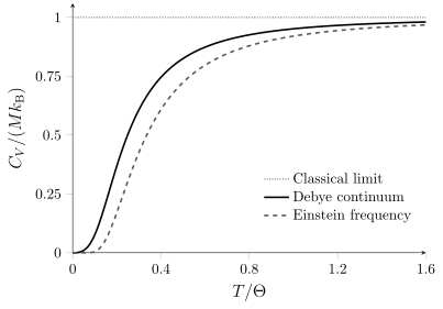
Complete model curves for equal mode weights and $\Theta_D=\Theta_E=\Theta$. Every Debye frequency is at or below the Einstein frequency. Since an oscillator’s heat capacity decreases with frequency at fixed $T$, averaging over these lower frequencies gives the higher Debye curve. Equal temperature parameters do not imply equal mean or mean-square frequency. The dotted line is the classical limit.

The harmonic high-temperature limit is a limit of the model. It does not guarantee that a real crystal remains harmonic, at fixed volume, or even in the same phase up to temperatures large compared with every vibrational scale.

Dimension and dispersion determine the power law

A branch with $\omega=A|\mathbf q|^s$ in $d$ spatial dimensions has an integrated state count proportional to $\omega^{d/s}$. Let $p=d/s>0$ and normalize a cutoff model by

$$g_p(\omega)=\frac{pM\omega^{p-1}}{\omega_c^p}, \qquad 0<\omega<\omega_c.$$

With $\Theta_c=\hbar\omega_c/k_{\rm B}$, changing variables in the thermal integral gives

$$\frac{C_V}{Mk_{\rm B}} \simeq p\,\Gamma(p+2)\zeta(p+1) \left(\frac{T}{\Theta_c}\right)^p.$$

Here $\Gamma$ is the gamma function and $\zeta$ the Riemann zeta function. The result follows by expanding $e^x/(e^x-1)^2=\sum_{m\geq1}m e^{-mx}$ and integrating each term. A two-dimensional linear branch has $C_V\propto T^2$; an ideal tension-free quadratic flexural branch has $C_V\propto T$. A finite system has a lowest nonzero frequency, tension can change flexural dispersion, and a layered solid can cross to three-dimensional behavior at low energy. A measured power law must therefore specify its size, coupling and dispersion window. Departure from $T^3$ is not automatically evidence for an Einstein optical mode.

Mixed reductions and what a fit preserves

A positive mixed spectrum has the form

$$\begin{gathered} g(\omega)=M_Dp_D(\omega) +\sum_j M_j\delta(\omega-\omega_j),\\ M_D+\sum_jM_j=3r,\qquad M_D,M_j\geq0, \end{gathered}$$

where $p_D=3\omega^2/\omega_D^3$ on its support is normalized to one. The free energy, internal energy and heat capacity are sums of their component contributions. A literal acoustic/optical interpretation fixes $M_D=3$ and $\sum_jM_j=3r-3$. More general phenomenological weights need not be integers, but then a Debye weight is not automatically the count of the three acoustic branches.

Different temperatures probe different information. The leading low-temperature power tests the lowest-frequency measure. The classical plateau tests the total weight. The leading high-temperature correction tests a second moment. None of these alone fixes the locations and weights of all optical states. Even matching all three leaves room for different intermediate-temperature curves, as Exercise 3 demonstrates.

In a finite, noisy temperature window, several spectra can give nearly indistinguishable heat-capacity curves. A fitted Einstein peak may summarize broad spectral weight rather than identify a single mode. Correlated parameter uncertainties and sensitivity to the number of components reveal this ambiguity; independent spectroscopy can constrain it. This practical limitation does not establish nonuniqueness for ideal, exact $C_V(T)$ at every temperature.

The appropriate spectral comparison uses an unweighted phonon DOS with the same thermal kernel and normalization. Scattering intensities contain matrix-element and species weights; Phonons explains why a generalized neutron DOS is not automatically the thermodynamic measure. Heat capacity also does not determine velocities, lifetimes or thermal conductivity. Heat Capacity and Thermodynamics explains how $C_p$ differs from $C_V$ and how electronic, magnetic, nuclear, defect and apparatus contributions enter a measurement.

Exercises

1. The same acoustic coefficient with two cutoffs

A primitive cell has two atoms. An acoustic-only Debye reduction assigns three modes a temperature $\Theta_A=180\,\mathrm K$. Keeping the same measured low-frequency DOS, find the temperature of an all-mode Debye reduction. Compare the two high-temperature plateaus. What fails if six Debye modes are instead assigned the original $180\,\mathrm K$ cutoff?

Solution

The low-frequency coefficient requires $M_D/\Theta_D^3$ to remain fixed. Thus

$$\Theta_{\rm all}=2^{1/3}\Theta_A \simeq226.786\,\mathrm K.$$

The acoustic subset tends to $3k_{\rm B}$ per cell and the all-mode model to $6k_{\rm B}$. The former needs three optical modes to represent the full crystal. Six modes at $180\,\mathrm K$ would double the acoustic coefficient and low-temperature $T^3$ heat capacity. A cutoff is meaningful only together with its assigned count.

2. Match one spectral moment, lose another

For equal mode weights, choose $\Theta_E$ so that an Einstein model has the same leading high-temperature heat-capacity correction as a Debye model of temperature $\Theta_D$. Does that also match their zero-point energies? Connect the test to $U=F-T\partial_TF$.

Solution

The correction measures the mean-square frequency. Equating the two coefficients gives

$$\frac{\Theta_E^2}{12}=\frac{\Theta_D^2}{20}, \qquad \Theta_E=\sqrt{\frac35}\,\Theta_D.$$

Matching the zero-point energy instead requires $\Theta_E/2=3\Theta_D/8$, or $\Theta_E=3\Theta_D/4$. Since $\sqrt{3/5}\ne3/4$, one Einstein frequency cannot satisfy both constraints. The zero-point constant is retained equally in $U$ and $F$, so the thermodynamic identity holds in either model, while its temperature derivative drops out of $C_V$. See Thermodynamic Potentials for that identity’s general meaning. Agreement of heat-capacity moments is not agreement of absolute vibrational energies.

3. Equal asymptotes, unequal intermediate curves

Use the two-atom cell of Exercise 1 and the same three-mode acoustic component at $180\,\mathrm K$ in both models. Model A adds three Einstein modes at $300\,\mathrm K$. Model B adds one at $100\,\mathrm K$ and two at $100\sqrt{13}\,\mathrm K$. Show that both have the same leading low-temperature law, classical plateau and $T^{-2}$ high-temperature correction. Evaluate $C_V/k_{\rm B}$ at $60$ and $120\,\mathrm K$ to test whether those constraints determine the curve.

Solution

Both spectra are positive and have six modes per cell. Their identical acoustic part dominates as $T\to0$, with

$$\frac{C_V}{k_{\rm B}T^3} \longrightarrow4.00860\times10^{-5}\,\mathrm{K^{-3}}.$$

The optical second moment in temperature units is $3(300)^2=(100)^2+2(100\sqrt{13})^2=270000\,\mathrm{K^2}$. Adding the acoustic contribution $3(3/5)(180)^2$ gives $328320\,\mathrm{K^2}$. Hence both have

$$\frac{C_V}{k_{\rm B}} =6-\frac{27360\,\mathrm{K^2}}{T^2}+O(T^{-4}).$$

The full integrals nevertheless give different values:

Temperature	Model A: $C_V/k_{\rm B}$	Model B: $C_V/k_{\rm B}$
$60\,\mathrm K$	$2.50050$	$2.96396$
$120\,\mathrm K$	$4.51452$	$4.62246$

Model B has more low-lying optical weight. Its difference from A first enters the high-temperature expansion at $T^{-4}$: the optical fourth-moment difference is $9.6\times10^9\,\mathrm{K^4}$, so $(C_B-C_A)/k_{\rm B}\simeq4.0\times10^7\,\mathrm{K^4}/T^4$. The shared asymptotes do not identify the spectral measure; sufficiently precise intermediate-temperature data distinguish these particular candidates.

4. A flexural branch is not an Einstein peak

For one two-dimensional branch with $\omega=Aq^2$, normalize its cutoff DOS to $M$ modes. Derive its leading low-temperature heat capacity. State the frequency window needed in a finite membrane and what changes if tension makes the long-wavelength dispersion linear.

Solution

Here $p=d/s=1$, so $g=M/\omega_c$ below the cutoff. The kernel gives

$$C_V\simeq\frac{\pi^2}{3}Mk_{\rm B} \frac{T}{\Theta_c}, \qquad \Theta_c=\frac{\hbar\omega_c}{k_{\rm B}}.$$

The power-law window requires the thermally populated frequencies to lie above the lowest nonzero finite-size mode and below the cutoff, with quadratic dispersion throughout the relevant range. A tension-induced linear regime instead has $p=2$ and a $T^2$ law there. Neither behavior is activated. Fitting a noncubic law with positive Einstein peaks over a short interval does not establish gapped microscopic oscillators.

References

• P. Debye, “Zur Theorie der spezifischen Wärmen,” Annalen der Physik 344, 789–839 (1912), doi:10.1002/andp.19123441404.
• A. Einstein, “Die Plancksche Theorie der Strahlung und die Theorie der spezifischen Wärme,” Annalen der Physik 327, 180–190 (1907), doi:10.1002/andp.19063270110.
• Phonopy developers, “Formulations: Thermodynamic properties,” official documentation, accessed 14 October 2026 — fixed-spectrum energy, Helmholtz free energy and constant-volume heat capacity.