Bose–Einstein Statistics

Bose–Einstein statistics gives the equilibrium occupation of ideal bosonic modes. For a mode $i$ with one-particle energy $\epsilon_i$ at positive temperature,

$$\overline n_i = \frac{1}{ e^{\beta(\epsilon_i-\mu)}-1 }, \qquad \beta = \frac{1}{k_{\mathrm B}T}.$$

The minus sign in the denominator is not a convention. It follows from the unrestricted bosonic occupation numbers

$$n_i = 0,1,2,\ldots.$$

For the ordinary grand-canonical sum to converge, every included mode must satisfy

$$\epsilon_i-\mu > 0.$$

In particular, for a finite ideal system with lowest one-particle energy $\epsilon_0$,

$$\mu < \epsilon_0.$$

The formula card gives the compact expression. The derivation below shows why the full occupation distribution is geometric and how it differs from a coherent state.

Helpful background. Bosonic Fock space supplies the number states; grand-canonical equilibrium supplies their statistical weights.

Bosonic modes and equilibrium weights

For ideal modes, take $H=\sum_i\epsilon_i n_i$ and $N=\sum_i n_i$. Symmetric exchange permits unrestricted occupations, but does not determine their probabilities. Combining those occupations with grand-canonical equilibrium weights gives the Bose–Einstein law. A coherent, squeezed, or number state is also bosonic and can have a very different number distribution.

The derivation requires independent modes and a convergent trace. In a quadratic quasiparticle approximation, identify whether it is $H$ or $H-\mu N$ that has been diagonalized; quasiparticle energies from the latter already include the chemical-potential dependence. For interacting bare particles the simple mode factorization generally fails.

Grand-Canonical Derivation

Introduce the grand Hamiltonian

$$K = H-\mu N.$$

For independent modes,

$$K = \sum_i (\epsilon_i-\mu)n_i.$$

Because the mode number operators commute, the grand partition function factorizes:

$$\Xi = \prod_i \xi_i.$$

For one bosonic mode,

$$\begin{aligned} \xi_i &= \sum_{n_i=0}^{\infty} e^{-\beta(\epsilon_i-\mu)n_i} \\ &= \sum_{n_i=0}^{\infty} q_i^{n_i}, \end{aligned}$$

where

$$q_i \equiv e^{-\beta(\epsilon_i-\mu)}.$$

If $0\leq q_i<1$, the geometric series gives

$$\xi_i = \frac{1}{1-q_i}.$$

The mean occupation follows from a logarithmic derivative:

$$\begin{aligned} \overline n_i &= q_i \frac{\partial}{\partial q_i} \ln\xi_i \\ &= \frac{q_i}{1-q_i}. \end{aligned}$$

Substituting the definition of $q_i$ yields

$$\overline n_i = \frac{1}{ e^{\beta(\epsilon_i-\mu)}-1 }.$$

The full ideal-mode grand potential is therefore

$$\Omega_{\mathrm G} = k_{\mathrm B}T \sum_i \ln \left[ 1-e^{-\beta(\epsilon_i-\mu)} \right].$$

Thermodynamic sums follow by differentiating this potential. For infinitely many modes, one also needs $\sum_i-\ln(1-q_i)<\infty$ to normalize this global Fock-space density operator. Convergence of each factor alone is insufficient; infinite-volume equilibrium is handled through thermodynamic limits rather than a normalized global product trace.

The Full One-Mode Distribution

The Bose–Einstein formula is a mean. The complete probability distribution for one ideal thermal mode is

$$P_i(n) = (1-q_i)q_i^n, \qquad n=0,1,2,\ldots.$$

Normalization follows from

$$\sum_{n=0}^{\infty} P_i(n) = (1-q_i) \sum_{n=0}^{\infty} q_i^n = 1.$$

Successive probabilities obey

$$\frac{P_i(n+1)}{P_i(n)} = q_i = e^{-\beta(\epsilon_i-\mu)}.$$

The distribution is geometric, not Poissonian. Expressed in terms of the mean,

$$q_i = \frac{\overline n_i}{1+\overline n_i},$$

so

$$P_i(n) = \frac{1}{1+\overline n_i} \left( \frac{\overline n_i}{1+\overline n_i} \right)^n.$$

Geometric and Poisson distributions

Writing $x=\beta(\epsilon-\mu)>0$ gives $f_{\mathrm B}=1/(e^x-1)$. The overview plot compares this mean with Bose, Fermi, and Boltzmann curves. To see information that the mean alone misses, compare a thermal mode and a Poisson law with the same mean:

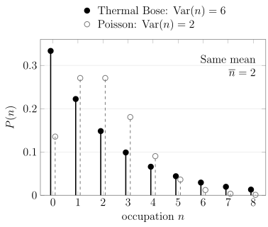
Both distributions have $\overline n=2$. The thermal law $P(n)=\frac13(\frac23)^n$ has variance six; the Poisson law $e^{-2}2^n/n!$ has variance two. The omitted tail $n\geq9$ contains about $2.60\%$ and $0.0237\%$ of their probabilities, respectively; the displayed points have not been renormalized.

Occupation Enhancement

The geometric series can be expanded as

$$\overline n_i = q_i + q_i^2 + q_i^3 + \cdots.$$

The first term is the Maxwell–Boltzmann occupation. The positive higher powers are the equilibrium statistical correction associated with unrestricted bosonic occupation.

The same enhancement appears algebraically in creation-operator matrix elements:

$$a_i^\dagger \lvert n_i\rangle = \sqrt{n_i+1} \lvert n_i+1\rangle.$$

Transition probabilities generated by a linear creation operator therefore contain a factor $n_i+1$. This is often called Bose enhancement or stimulated emission.

The two statements are related by bosonic occupation algebra, but they answer different questions. The Bose–Einstein distribution is an equilibrium probability law; the factor $n+1$ in a transition rate is a dynamical matrix-element effect.

Fluctuations and Bunching

For the geometric distribution,

$$\langle n_i^2\rangle = \overline n_i + 2\overline n_i^2.$$

Hence

$$\operatorname{Var}(n_i) = \overline n_i \left( 1+\overline n_i \right).$$

The first term is the Poisson-like contribution. The second is the bosonic excess fluctuation.

The normally ordered second moment is

$$\langle n_i(n_i-1)\rangle = 2\overline n_i^2.$$

For one ideal thermal mode with nonzero mean, the normalized equal-time second-order coherence is

$$g^{(2)}(0) \equiv \frac{ \langle n_i(n_i-1)\rangle }{ \overline n_i^2 } = 2.$$

This is the ideal single-mode thermal bunching result. Multimode detection, finite time resolution, interactions, coherence, and detector response can change the observed value, so $g^{(2)}(0)=2$ is not a universal statement about every bosonic source.

The relative fluctuation is

$$\frac{ \sqrt{\operatorname{Var}(n_i)} }{ \overline n_i } = \sqrt{ 1+ \frac{1}{\overline n_i} }.$$

It approaches one, rather than zero, when one ideal thermal mode becomes highly occupied. Bulk thermodynamic relative fluctuations can still vanish after many modes or spatial cells are combined. A macroscopically occupied condensate mode requires special ensemble and interaction care.

Fluctuation–Response Identity

Differentiate the occupation with respect to chemical potential:

$$\left( \frac{\partial\overline n_i}{\partial\mu} \right)_T = \beta \overline n_i \left( 1+\overline n_i \right).$$

Therefore

$$\left( \frac{\partial\overline n_i}{\partial\mu} \right)_T = \beta \operatorname{Var}(n_i).$$

Similarly,

$$- \frac{1}{\beta} \left( \frac{\partial\overline n_i}{\partial\epsilon_i} \right)_{T,\mu} = \operatorname{Var}(n_i).$$

The sharp growth of occupation near $\epsilon_i=\mu$ is inseparable from enhanced mode-number fluctuations in the ideal grand-canonical description.

Approach to the Lowest Mode

Let

$$\delta \equiv \epsilon_0-\mu > 0.$$

Then

$$\overline n_0 = \frac{1}{e^{\beta\delta}-1}.$$

For $\beta\delta\ll1$,

$$\overline n_0 \sim \frac{1}{\beta\delta}.$$

The divergence signals that the lowest mode cannot always be treated as an ordinary thermodynamic correction. In a fixed-density ideal Bose gas, the chemical potential approaches $\epsilon_0$ from below and the ground-state occupation may become macroscopic.

That statement is a bridge to the ideal Bose gas and Bose–Einstein condensation. Whether condensation occurs, and how the excited-state population saturates, depends on the density of states, dimensionality, confinement, and thermodynamic limit.

Conserved and Nonconserved Boson Number

For conserved atoms described grand canonically, $\mu$ is adjusted so that

$$\overline N = \sum_i \overline n_i$$

matches the required mean particle number. An exactly fixed-number finite system instead uses a canonical trace; its occupations are correlated, and need not follow this independent-mode distribution.

For equilibrium excitations whose number is not conserved, the associated chemical potential is ordinarily zero. Important examples are photons in blackbody equilibrium and phonons in a crystal:

$$\mu_\gamma = 0, \qquad \mu_{\mathrm{ph}} = 0.$$

This is not a statement that every bosonic species has zero chemical potential. Conserved atoms generally have nonzero $\mu$, and driven or approximately conserved quasiparticle populations can sometimes be described by an effective chemical potential. Such a parameter must be justified by conservation laws and timescales.

High-Energy and Dilute Limit

When

$$x = \beta(\epsilon-\mu) \gg 1,$$

the occupation is small. Writing $y=e^{-x}$ gives

$$\begin{aligned} f_{\mathrm B}(x) &= \frac{y}{1-y} \\ &= y+y^2+y^3+\cdots. \end{aligned}$$

Therefore

$$f_{\mathrm B}(x) \simeq e^{-x}.$$

This is the Maxwell–Boltzmann limit. Classical Limit of Quantum Statistics turns this mode-level expansion into the homogeneous criterion $n\lambda_T^d/g\ll1$ and derives the unified Bose/Fermi virial correction. The leading relative correction here is of order $e^{-x}$:

$$\frac{ f_{\mathrm B}(x)-e^{-x} }{ e^{-x} } = e^{-x} + O(e^{-2x}).$$

Quantum statistics becomes negligible mode by mode when every relevant occupation is much less than one. In a gas, that condition is commonly expressed through low fugacity or a small phase-space density.

Highly Occupied Limit

For $x\ll1$ with $x>0$,

$$\frac{1}{e^x-1} = \frac{1}{x} - \frac{1}{2} + \frac{x}{12} - \frac{x^3}{720} + O(x^5).$$

The leading term is

$$\overline n \simeq \frac{k_{\mathrm B}T}{\epsilon-\mu}.$$

This is the classical-field or Rayleigh–Jeans form for a highly occupied mode. Applying it to arbitrarily high energies produces ultraviolet divergences; the full Bose–Einstein denominator supplies the quantum suppression at large $x$.

Zero-Temperature Limit

At fixed $\mu<\epsilon_0$,

$$\lim_{T\to0^+} \overline n_i = 0$$

for every included mode.

That limit is not the correct fixed-particle-number limit for a Bose gas with particles present. At fixed $N$, the chemical potential generally changes with temperature and can approach the lowest one-particle energy. The ground mode must then be separated from the excited-state continuum.

The lesson is simple: a temperature limit is incomplete unless one states which thermodynamic variables are held fixed.

Mode Versus Degenerate Level

The Bose–Einstein formula gives occupation per mode. If an energy level $\epsilon$ has degeneracy $g_\epsilon$ and the modes are independent, then

$$\overline N_\epsilon = g_\epsilon f_{\mathrm B} \left[ \beta(\epsilon-\mu) \right].$$

The level variance is

$$\operatorname{Var}(N_\epsilon) = g_\epsilon \overline n_\epsilon \left( 1+\overline n_\epsilon \right)$$

when the degenerate modes fluctuate independently.

In a continuum approximation, sums become integrals over the one-particle density of states $g(\epsilon)$:

$$\overline N = \int d\epsilon\, g(\epsilon) \frac{1}{ e^{\beta(\epsilon-\mu)}-1 }.$$

The density of states controls whether the excited modes can hold an arbitrarily large density. This is where dimensionality enters the theory of ideal-gas condensation.

Entropy Per Mode

For a geometric thermal mode, the von Neumann entropy can be written entirely in terms of $\overline n$:

$$\frac{s_{\mathrm B}}{k_{\mathrm B}} = \left( 1+\overline n \right) \ln \left( 1+\overline n \right) - \overline n \ln\overline n.$$

This expression follows by substituting the geometric probabilities into

$$s = -k_{\mathrm B} \sum_n P(n)\ln P(n).$$

It vanishes as $\overline n\to0$ and grows logarithmically for large occupation. Summing it over independent modes gives the entropy of an ideal bosonic gas or a collection of independent thermal oscillators.

Example: One Harmonic-Oscillator Mode

For one oscillator of angular frequency $\omega$,

$$H = \hbar\omega \left( n+\frac{1}{2} \right).$$

If oscillator quanta are not conserved, $\mu=0$. The mean excitation number is

$$\overline n = \frac{1}{e^{\beta\hbar\omega}-1}.$$

The mean energy is

$$U = \hbar\omega \left( \overline n+\frac{1}{2} \right).$$

The zero-point term does not affect the normalized occupation probabilities. The heat capacity is

$$C = k_{\mathrm B} (\beta\hbar\omega)^2 \frac{ e^{\beta\hbar\omega} }{ \left( e^{\beta\hbar\omega}-1 \right)^2 }.$$

At high temperature, $U=k_{\mathrm B}T+(\hbar\omega)^2/(12k_{\mathrm B}T)+\cdots$. The thermal excitation energy alone is $U-\hbar\omega/2=k_{\mathrm B}T-\hbar\omega/2+\cdots$; it agrees with equipartition only to leading relative order. At low temperature, thermal excitation is exponentially suppressed.

Example: Photons

Each electromagnetic normal mode is a bosonic oscillator. In blackbody equilibrium, photon number is not conserved, so

$$\mu_\gamma = 0.$$

For a mode with angular frequency $\omega$,

$$\overline n_\omega = \frac{1}{e^{\beta\hbar\omega}-1}.$$

Multiplying the mean energy per mode by the electromagnetic density of states and polarization degeneracy produces Planck’s radiation law. Planck’s Radiation Law derives the spectrum and explains its experimental role.

Example: Phonons

In a harmonic crystal, each normal mode with branch label $s$ and wavevector $\mathbf k$ has mean occupation

$$\overline n_{\mathbf k s} = \frac{1}{ e^{\beta\hbar\omega_{\mathbf k s}}-1 }.$$

Equilibrium phonon number is not conserved, so the phonon chemical potential is zero. Exact rigid-translation zero modes must be handled separately, for example by fixing the crystal center of mass or its boundaries; inserting $\omega=0$ into a harmonic-oscillator geometric sum does not give a normalizable state. Summing $\hbar\omega_{\mathbf k s}\overline n_{\mathbf k s}$ over the phonon density of states gives the thermal lattice energy in the harmonic approximation. Phonons as Many-Body Excitations derives the modes, operators, zero-point term, and displacement correlations behind this statistical description.

The low-temperature power law depends on the acoustic dispersion and spatial dimension; the high-temperature limit approaches classical equipartition over thermally accessible modes.

Interactions and Quasiparticles

For interacting bosons, the microscopic Hamiltonian need not be diagonal in the original occupation numbers. Then

$$H \neq \sum_i \epsilon_i n_i$$

in the basis of bare one-particle modes, and the independent geometric-mode derivation fails.

A quadratic effective Hamiltonian may sometimes be diagonalized into bosonic quasiparticles:

$$H_{\mathrm{eff}} = E_0 + \sum_\alpha E_\alpha b_\alpha^\dagger b_\alpha.$$

If those quasiparticles equilibrate and their number is not conserved, then

$$\overline n_\alpha = \frac{1}{e^{\beta E_\alpha}-1}.$$

This does not mean the original particle occupations have the same simple distribution. One must identify which modes diagonalize the effective theory and which conserved charges determine their chemical potentials.

Fixed number and the condensation limit

For a finite ideal system, the convergence condition is strict:

$$\mu < \epsilon_0.$$

All occupations are finite for finite $T$ and finite separation $\epsilon_0-\mu$.

A sharp condensation transition is a thermodynamic-limit statement. In a finite trap or box, observables vary smoothly and the lowest-mode occupation can become large without a mathematical nonanalyticity.

Grand-canonical fluctuations of an ideal condensate can also be anomalously large. Fixed-$N$ constraints and interactions alter those fluctuations. The ideal Bose gas develops the excited-state sum and Bose–Einstein condensation analyzes macroscopic occupation. Their finite-number fluctuations need their specified ensemble.

Evaluating small gaps and probability tails

For small positive $x=\beta(\epsilon-\mu)$, evaluate $f=1/\operatorname{expm1}(x)$ to avoid cancellation in $e^x-1$. At large $x$, $e^{-x}/(1-e^{-x})$ avoids overflow. If a numerical probability sum stops at $n_{\max}$, the exact omitted mass is

$$\Pr(n>n_{\max})=q^{n_{\max}+1}.$$

Choose the cutoff from this tail probability, rather than from the mean alone; highly occupied geometric distributions have broad tails.

Exercises

Derive the mode variance

Starting from $\overline n=q/(1-q)$, show that

$$\operatorname{Var}(n) = \overline n(1+\overline n).$$

Solution

For a geometric distribution,

$$\operatorname{Var}(n) = q \frac{\partial\overline n}{\partial q}.$$

Since

$$\frac{\partial}{\partial q} \left( \frac{q}{1-q} \right) = \frac{1}{(1-q)^2},$$

one obtains

$$\operatorname{Var}(n) = \frac{q}{(1-q)^2}.$$

Also,

$$\begin{aligned} \overline n(1+\overline n) &= \frac{q}{1-q} \left( 1+\frac{q}{1-q} \right) \\ &= \frac{q}{(1-q)^2}. \end{aligned}$$

Thus the two expressions agree.

Count a degenerate level

An energy level $\epsilon$ contains $g$ independent bosonic modes. Find its mean total occupation and variance.

Solution

Every mode has the same mean

$$\overline n = \frac{1}{e^{\beta(\epsilon-\mu)}-1}.$$

The total level occupation is

$$N_\epsilon = \sum_{a=1}^{g} n_a.$$

Linearity gives

$$\overline N_\epsilon = g\overline n.$$

Independence makes the variances additive:

$$\operatorname{Var}(N_\epsilon) = g\overline n \left( 1+\overline n \right).$$

Degeneracy multiplies the number of modes; it does not change the mean occupation of each mode.

Recover the oscillator heat capacity

For a bosonic oscillator mode with $\mu=0$, derive the heat capacity from

$$U = \hbar\omega \left[ \frac{1}{e^{\beta\hbar\omega}-1} + \frac{1}{2} \right].$$

Check the high- and low-temperature limits.

Solution

Let

$$x = \beta\hbar\omega.$$

Since

$$\frac{dx}{dT} = - \frac{x}{T},$$

differentiation gives

$$C = k_{\mathrm B}x^2 \frac{e^x}{(e^x-1)^2}.$$

For $x\ll1$,

$$\frac{e^x}{(e^x-1)^2} \sim \frac{1}{x^2},$$

so

$$C \longrightarrow k_{\mathrm B}.$$

For $x\gg1$,

$$C \sim k_{\mathrm B}x^2e^{-x},$$

which vanishes exponentially. The temperature-independent zero-point energy contributes nothing to $C$.

Two modes with a fixed total

Two equal-energy bosonic modes contain exactly $N=2$ particles. Find the probability law, mean, and variance of $n_1$. Compare its variance with a geometric law of the same mean.

Solution

The three Fock states $(2,0)$, $(1,1)$, and $(0,2)$ have the same energy and equal canonical probability $1/3$. Thus $n_1=0,1,2$ is uniform, with mean one and variance $(0+1+4)/3-1=2/3$. A geometric mode with mean one has variance two. Fixing the total number changes the distribution even in this noninteracting example.

Unresolved independent thermal modes

A detector sums $g$ independent thermal bosonic modes, each with mean $f>0$. Show that its normalized factorial moment is $\langle N(N-1)\rangle/\langle N\rangle^2=1+1/g$.

Solution

Each mode contributes $\langle n_a(n_a-1)\rangle=2f^2$, and each ordered distinct pair contributes $\langle n_an_b\rangle=f^2$. Therefore

$$\langle N(N-1)\rangle=2gf^2+g(g-1)f^2=g(g+1)f^2.$$

Since $\langle N\rangle=gf$, division gives $1+1/g$. Unresolved modes reduce the bunching contrast even though each individual thermal mode has normalized factorial moment two. Unequal means replace $1/g$ by $\sum_a f_a^2/(\sum_a f_a)^2$.

References

• A. L. Fetter and J. D. Walecka, Quantum Theory of Many-Particle Systems, Dover (2003).
• K. Huang, Statistical Mechanics, 2nd ed., Wiley (1987).
• M. Kardar, Statistical Physics of Particles, Cambridge University Press (2007).
• L. D. Landau and E. M. Lifshitz, Statistical Physics, Part 1, 3rd ed., Butterworth–Heinemann (1980).
• L. Mandel and E. Wolf, Optical Coherence and Quantum Optics, Cambridge University Press (1995).
• R. K. Pathria and P. D. Beale, Statistical Mechanics, 3rd ed., Elsevier (2011).
• C. J. Pethick and H. Smith, Bose–Einstein Condensation in Dilute Gases, 2nd ed., Cambridge University Press (2008).
• L. Pitaevskii and S. Stringari, Bose–Einstein Condensation and Superfluidity, Oxford University Press (2016).