Weakly Interacting Bose Gas Preview

A weakly interacting Bose gas is a dilute gas of bosons whose low-energy two-body collisions are important but whose many-body correlations remain perturbatively small. In three dimensions, the standard control parameter is the gas parameter

$$\gamma = n a_s^3 \ll 1,$$

where $n=N/V$ is the number density and $a_s$ is the $s$-wave scattering length. The phrase weakly interacting does not mean that a dimensional coupling constant is numerically small by itself. It means that the interaction length is much smaller than the mean interparticle spacing:

$$a_s \ll n^{-1/3}.$$

Even in this controlled regime, interactions change the infrared physics qualitatively. The ideal condensate has quadratic excitations, zero interaction pressure, divergent compressibility, and no nonzero Landau critical velocity. A weak repulsion produces a finite chemical potential, a healing length, and a linear sound branch. It also depletes the condensate at zero temperature and shifts the ground-state energy beyond mean field.

We connect the dilute-gas equation of state to sound, depletion, and the first correction beyond mean field. The Gross–Pitaevskii equation develops spatial mean fields, while Bogoliubov theory gives the systematic quadratic diagonalization. The point here is to see which physical scale each result predicts and which approximation makes it reliable.

Helpful background. Bose condensation defines the condensate, and field operators explains the Hamiltonian and normalization.

A dilute gas with a matched short-range interaction

Unless stated otherwise, consider:

• one species of spinless bosons;
• three spatial dimensions;
• a homogeneous volume $V$ with periodic boundary conditions;
• short-range, repulsive interactions;
• positive scattering length $a_s>0$;
• zero temperature, or temperatures low enough that condensate depletion is small;
• the thermodynamic limit at fixed density;
• wavelengths long compared with the microscopic interaction range.

A positive scattering length alone does not prove that a microscopic potential is repulsive or that an atomic gas is the absolute ground state: bound molecules may exist. We assume a stable repulsive gas, or a sufficiently long-lived atomic branch whose losses can be neglected on the timescale studied. The low-energy Hamiltonian is

$$\hat H ={} \int d^3r\, \frac{\hbar^2}{2m} \boldsymbol\nabla\hat\psi^\dagger \boldsymbol\cdot \boldsymbol\nabla\hat\psi + \frac{g}{2} \int d^3r\, \hat\psi^\dagger \hat\psi^\dagger \hat\psi \hat\psi,$$

with equal-time commutator

$$[ \hat\psi(\mathbf r), \hat\psi^\dagger(\mathbf r') ] = \delta^{(3)}(\mathbf r-\mathbf r').$$

At leading order in the low-energy expansion,

$$g = \frac{4\pi\hbar^2 a_s}{m}.$$

This formula uses the physical, renormalized scattering length. A bare coefficient multiplying a delta function depends on the ultraviolet prescription once loop or zero-point integrals are evaluated. It must not be identified with $4\pi\hbar^2a_s/m$ at every cutoff without matching.

Why Scattering Length Is the Right Input

Let $U(r)$ be a short-range microscopic two-body potential. At low relative momentum, its $s$-wave phase shift obeys the effective-range expansion

$$k\cot\delta_0(k) = -\frac{1}{a_s} + \frac{r_e}{2}k^2 + O(k^4),$$

where $r_e$ is the effective range. The scattering amplitude is

$$f_0(k) = \frac{1}{ k\cot\delta_0(k)-ik }.$$

Keeping only scattering-length data requires the effective-range term to be small compared with the retained inverse-amplitude terms:

$$\frac{|r_e|k^2}{2}\ll|-a_s^{-1}-ik|.$$

One also needs momenta below the inverse microscopic range $R^{-1}$ and below other internal-channel thresholds. In the regime $k a_s\ll1$, a useful sufficient range condition is $|a_s r_e|k^2\ll1$; the statement $k|r_e|\ll1$ alone is not the complete matching criterion. An energy-independent leading coupling $g$ is appropriate on these low-energy scales.

This two-body reduction and the many-body condition $na_s^3\ll1$ are distinct. For the typical collective momentum $k\sim\xi^{-1}$ below, $ka_s\sim\sqrt{8\pi na_s^3}$ becomes small in the dilute limit, but an anomalously large effective range or a nearby channel can introduce another restriction. The contact model is a low-energy representation, not a microscopic point-particle assertion.

Momentum-Space Hamiltonian

For a periodic box,

$$\hat\psi(\mathbf r) = \frac{1}{\sqrt V} \sum_{\mathbf k} e^{i\mathbf k\cdot\mathbf r} \hat a_{\mathbf k},$$

and

$$\epsilon_k = \frac{\hbar^2k^2}{2m}.$$

The Hamiltonian becomes

$$\hat H ={} \sum_{\mathbf k} \epsilon_k \hat a_{\mathbf k}^\dagger \hat a_{\mathbf k} + \frac{g}{2V} \sum_{\mathbf k,\mathbf k',\mathbf q} \hat a_{\mathbf k+\mathbf q}^\dagger \hat a_{\mathbf k'-\mathbf q}^\dagger \hat a_{\mathbf k'} \hat a_{\mathbf k}.$$

The wave-vector transfer $\mathbf q$ (physical momentum transfer $\hbar\mathbf q$) redistributes momentum between two particles while preserving total momentum. Unlike the ideal-gas Hamiltonian, the interaction does not commute with each individual mode occupation. Momentum modes are coupled, and the exact eigenstates are not single occupation-number configurations.

Mean-Field Ground-State Energy

Start with the idealized state in which all $N$ particles occupy the zero-momentum mode:

$$|N_0=N\rangle = \frac{ (\hat a_{\mathbf0}^\dagger)^N }{\sqrt{N!}} |0\rangle.$$

Its kinetic energy is zero. The interaction expectation value uses

$$\left\langle \hat a_{\mathbf0}^\dagger \hat a_{\mathbf0}^\dagger \hat a_{\mathbf0} \hat a_{\mathbf0} \right\rangle = N(N-1),$$

so

$$E_{\mathrm{MF}} = \frac{g}{2V} N(N-1).$$

In the thermodynamic limit,

$$\frac{E_{\mathrm{MF}}}{V} = \frac{g}{2}n^2.$$

The factor $1/2$ prevents double counting of particle pairs. This is the leading matched contact-theory mean-field expectation, not an exact microscopic-potential energy. The trial state neglects the pair correlations generated by interactions.

Equation of State

At fixed volume, the mean-field chemical potential is

$$\mu_{\mathrm{MF}} = \left( \frac{\partial E_{\mathrm{MF}}}{\partial N} \right)_V = gn$$

in the thermodynamic limit. The pressure is

$$P_{\mathrm{MF}} = -\left( \frac{\partial E_{\mathrm{MF}}}{\partial V} \right)_N = \frac{g}{2}n^2.$$

The isothermal compressibility at zero temperature is

$$\kappa_T = \frac{1}{n} \left( \frac{\partial n}{\partial P} \right)_T = \frac{1}{gn^2}.$$

Thus an arbitrarily weak positive $g$ gives the condensate a finite inverse compressibility. In the ideal limit $g\to0^+$,

$$\kappa_T \to \infty.$$

The Chemical Potential page explains why $\mu$ is an addition-energy derivative rather than the energy of a distinguished particle.

Mean Field as a Condensate Amplitude

Introduce a condensate amplitude $\Phi(\mathbf r)$ normalized by

$$\int d^3r\, |\Phi(\mathbf r)|^2 = N.$$

At this leading order condensate number is approximated by total number. The corresponding energy functional is

$$E[\Phi] = \int d^3r\, \left[ \frac{\hbar^2}{2m} |\boldsymbol\nabla\Phi|^2 + V_{\mathrm{ext}} |\Phi|^2 + \frac{g}{2} |\Phi|^4 \right].$$

Stationarity at fixed particle number gives the signpost equation

$$\left[ -\frac{\hbar^2\nabla^2}{2m} + V_{\mathrm{ext}} + g|\Phi|^2 \right] \Phi = \mu\Phi.$$

For a uniform condensate, $\Phi=\sqrt n$ and $\mu=gn$. Gross–Pitaevskii Equation derives this equation carefully, distinguishes stationary and time-dependent formulations, and treats boundary conditions, vortices, and trapped profiles. Here it serves only to show how the uniform equation of state enters a spatially varying condensate.

Replacing an operator by a complex amplitude is a representation of mean-field order, not an exact operator identity. Exact finite-$N$ states can preserve particle-number symmetry; number-conserving formulations reproduce the leading results without assigning a nonzero expectation value to $\hat\psi$.

Interaction Scales

Three scales organize the weakly interacting gas.

Interaction energy

The mean-field energy per added particle is

$$\mu = gn.$$

This separates the collective low-energy regime from approximately single-particle behavior.

Sound speed

At zero temperature, hydrodynamics gives

$$c^2 = \frac{1}{m} \frac{\partial P}{\partial n}.$$

Using the mean-field pressure,

$$c = \sqrt{\frac{gn}{m}}.$$

Equivalently,

$$mc^2 = gn.$$

Healing length

Balance the kinetic cost of varying the condensate over a distance $\xi$ against the interaction energy:

$$\frac{\hbar^2}{2m\xi^2} = gn.$$

The Gross–Pitaevskii healing-length convention used here is

$$\xi = \frac{\hbar}{\sqrt{2mgn}} = \frac{1}{\sqrt{8\pi n a_s}}.$$

It obeys

$$\xi = \frac{\hbar}{\sqrt{2}\,mc}.$$

Different texts sometimes absorb the factor $\sqrt2$ into the definition of a coherence or healing length. Always check the defining balance before comparing formulas.

Parametrically, the dilute limit generates the hierarchy

$$a_s \ll n^{-1/3} \ll \xi,$$

up to numerical factors. The first inequality suppresses short-range many-body encounters; the second allows collective density variations to involve many particles.

Why the Ideal Excitation Spectrum Fails

For the ideal gas,

$$E_k^{(0)} = \epsilon_k = \frac{\hbar^2k^2}{2m}.$$

The phase velocity tends to zero:

$$\frac{E_k^{(0)}}{\hbar k} = \frac{\hbar k}{2m} \longrightarrow 0$$

as $k\to0$. A fluid with this spectrum has no positive Landau threshold for creating excitations. The same softness appears thermodynamically as infinite compressibility below the ideal-gas condensation temperature.

Interactions cannot be represented merely by adding a constant Hartree shift to every excitation. Particle and hole amplitudes mix, and that mixing is what produces a gapless collective branch.

Bogoliubov Expansion Preview

Work with the grand-canonical operator

$$\hat K = \hat H - \mu\hat N.$$

When the zero-momentum mode is macroscopically occupied, write schematically

$$\hat a_{\mathbf0} \approx \sqrt{N_0}$$

and retain terms through quadratic order in $\hat a_{\mathbf k\ne0}$. The stationary condensate condition

$$\mu = gn_0, \qquad n_0 = \frac{N_0}{V},$$

makes the energy stationary under a change of the condensate amplitude. In a uniform expansion restricted to nonzero momenta, translation invariance already forbids linear terms in those modes. The quadratic fluctuation Hamiltonian is

$$\hat K_2 ={} \sum_{\mathbf k\ne\mathbf0} \Bigg[ (\epsilon_k+gn_0) \hat a_{\mathbf k}^\dagger \hat a_{\mathbf k} + \frac{gn_0}{2} \left( \hat a_{\mathbf k}^\dagger \hat a_{-\mathbf k}^\dagger + \hat a_{\mathbf k} \hat a_{-\mathbf k} \right) \Bigg].$$

The anomalous terms exchange opposite-momentum atom pairs with the condensate represented by its amplitude. The underlying Hamiltonian conserves total particle number. Therefore bare particles of momentum $\mathbf k$ are not the normal modes.

The approximation organizes the Hamiltonian as:

Order in fluctuations	Role
no fluctuation operators	condensate mean-field energy
one fluctuation operator	vanishes when the background is stationary
two fluctuation operators	independent quasiparticles after diagonalization
three and four fluctuation operators	quasiparticle interactions neglected at leading order

The actual control condition is small depletion and weak quasiparticle interactions, not a formal claim that every higher-power operator is always negligible.

Particle–Hole Mixing

Introduce quasiparticle operators by

$$\hat a_{\mathbf k} = u_k\hat b_{\mathbf k} - v_k\hat b_{-\mathbf k}^\dagger,$$

with real coefficients satisfying

$$u_k^2-v_k^2 = 1.$$

This condition preserves the bosonic commutator. For repulsive $g$ and this minus-sign convention, choose $u_k,v_k\ge0$, with $u_kv_k=gn_0/(2E_k)$. Their squares are

$$u_k^2 = \frac12 \left( \frac{\epsilon_k+gn_0}{E_k} + 1 \right),$$

and

$$v_k^2 = \frac12 \left( \frac{\epsilon_k+gn_0}{E_k} - 1 \right).$$

The resulting excitation energy is

$$E_k = \sqrt{ \epsilon_k (\epsilon_k+2gn_0) }.$$

At leading order in the dilute expansion, one may replace $n_0$ by $n$ inside this spectrum. Their difference is already of relative order $\sqrt{na_s^3}$.

The quasiparticle vacuum is not the state with every atom in the zero-momentum mode. It is a correlated, pair-squeezed state with nonzero occupation $v_k^2$ in modes $\mathbf k\ne0$.

Bogoliubov Quasiparticles compares this bosonic hyperbolic mixing with fermionic pairing and explains how $u_k$ and $v_k$ enter particle content, conserved quantities, and probe coherence factors.

A Two-by-Two View of the Spectrum

The equations of motion for the pair

$$\begin{pmatrix} \hat a_{\mathbf k} \\ \hat a_{-\mathbf k}^\dagger \end{pmatrix}$$

involve the matrix

$$\mathcal L_k = \begin{pmatrix} \epsilon_k+gn_0 & gn_0 \\ -gn_0 & -(\epsilon_k+gn_0) \end{pmatrix}.$$

Its eigenvalues satisfy

$$\lambda_k^2 = (\epsilon_k+gn_0)^2 -(gn_0)^2,$$

and hence

$$\lambda_k = \pm E_k.$$

The minus sign in the lower row reflects the bosonic particle–hole metric. This is why diagonalizing the ordinary symmetric coefficient matrix as though it were a one-particle Hamiltonian gives the wrong answer.

Collective and Particle-Like Regimes

Define

$$q = k\xi.$$

Because

$$\epsilon_k = gnq^2,$$

the leading spectrum takes the universal dimensionless form

$$\frac{E_k}{gn} = \sqrt{ q^2(q^2+2) }.$$

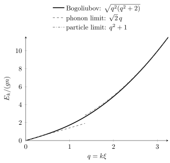
The Bogoliubov dispersion in units set by $gn$ and the healing length $\xi=\hbar/\sqrt{2mgn}$. For $k\xi\ll1$, $E_k/(gn)\simeq\sqrt{2}\,k\xi$; for $k\xi\gg1$, $E_k/(gn)\simeq(k\xi)^2+1$.

Long wavelengths

For $q\ll1$,

$$E_k = \hbar ck \left[ 1 + \frac{(k\xi)^2}{4} + O((k\xi)^4) \right].$$

The excitations are phonons: collective density and phase waves rather than atoms carrying a definite momentum independently of the medium.

Shorter wavelengths

For $q\gg1$ while the contact description remains valid,

$$E_k = \epsilon_k + gn - \frac{(gn)^2}{2\epsilon_k} + O(\epsilon_k^{-2}).$$

The excitation becomes particle-like, with a leading mean-field shift. This is an intermediate asymptotic statement: at momenta comparable to the inverse interaction range, the contact theory itself must be refined.

Crossover

The crossover occurs near

$$k\xi \sim 1,$$

or equivalently

$$\epsilon_k \sim gn.$$

The healing length is therefore both a spatial recovery scale and the wavelength separating collective from particle-like excitations.

Gaplessness and Symmetry

The microscopic Hamiltonian conserves total particle number and is invariant under

$$\hat\psi \longmapsto e^{i\alpha} \hat\psi.$$

In a thermodynamic symmetry-breaking description, the condensate chooses a phase. Long-wavelength phase variations cost arbitrarily little energy, producing the gapless phonon branch. The simple Bogoliubov spectrum indeed obeys

$$E_{k=0} = 0.$$

At finite size and fixed $N$, one can retain exact number symmetry. The same collective spectrum emerges through number-conserving constructions. A nonzero order-parameter expectation value is a useful thermodynamic representation, not the only logically possible formulation. The broader symmetry logic is introduced in Spontaneous Symmetry Breaking Preview.

Quantum Depletion

At zero temperature, the Bogoliubov quasiparticle vacuum satisfies

$$\langle \hat b_{\mathbf k}^\dagger \hat b_{\mathbf k} \rangle = 0,$$

but the atomic momentum modes have occupation

$$\langle \hat a_{\mathbf k}^\dagger \hat a_{\mathbf k} \rangle = v_k^2.$$

Thus the noncondensed density is

$$n_{\mathrm{ex}} = \int \frac{d^3k}{(2\pi)^3} v_k^2.$$

For the homogeneous three-dimensional dilute gas,

$$\frac{n_{\mathrm{ex}}}{n} = \frac{8}{3\sqrt\pi} \sqrt{na_s^3} + o(\sqrt{na_s^3}).$$

This is quantum depletion: it remains at $T=0$ and arises from interaction-induced pair correlations. It is distinct from thermal depletion. Small $\sqrt{na_s^3}$ makes the condensate fraction close to one, but never exactly one for a nonzero repulsive interaction in the thermodynamic ground state.

The Bose–Einstein Condensation page defines condensate occupation independently of basis. Here depletion is used as the quantitative diagnostic controlling the weak-correlation expansion.

Beyond Mean Field: Lee–Huang–Yang Term

The quadratic modes have zero-point energy. A naive contact-theory sum is ultraviolet divergent, so the bare coupling must be eliminated in favor of the physical scattering length before a finite result is quoted. After this matching, the ground-state energy density is

$$\frac{E}{V} = \frac{gn^2}{2} \left[ 1 + \frac{128}{15\sqrt\pi} \sqrt{na_s^3} + O\!\left( na_s^3\ln(na_s^3) \right) \right].$$

The leading correction is the Lee–Huang–Yang term. Differentiation gives

$$\mu = gn \left[ 1 + \frac{32}{3\sqrt\pi} \sqrt{na_s^3} + \cdots \right].$$

Several lessons are packed into these formulas:

1. Mean field is the first term of a controlled expansion, not an exact result.
2. The first correction is nonanalytic in $g$ when expressed at fixed density because $a_s\propto g$ at leading order.
3. The same parameter $\sqrt{na_s^3}$ controls both depletion and the leading energy correction.
4. Higher orders eventually depend on additional short-distance data as well as logarithms.

The Lee–Huang–Yang term is a standard established result for the dilute homogeneous three-dimensional gas. Applying a local version of it to mixtures, dipolar gases, low dimensions, or rapidly varying trapped profiles requires a new validity analysis.

Density Fluctuations and Structure Factor

For nonzero wave vector, define $\hat n_{\mathbf k}=\int_Vd^3r\,e^{-i\mathbf k\cdot\mathbf r}\hat\psi^\dagger(\mathbf r)\hat\psi(\mathbf r)$ and the fluctuation

$$\delta\hat n_{\mathbf k} = \hat n_{\mathbf k} - \langle\hat n_{\mathbf k}\rangle.$$

With the normalization

$$S(k) = \frac{1}{N} \left\langle \delta\hat n_{\mathbf k} \delta\hat n_{-\mathbf k} \right\rangle,$$

Bogoliubov theory at zero temperature gives

$$S(k) = \frac{\epsilon_k}{E_k}.$$

At long wavelength,

$$S(k) \sim \frac{\hbar k}{2mc}.$$

The vanishing of $S(k)$ as $k\to0$ shows that repulsive interactions suppress long-wavelength density fluctuations. At finite temperature within the quasiparticle approximation,

$$S(k) = \frac{\epsilon_k}{E_k} \coth\!\left( \frac{\beta E_k}{2} \right).$$

Taking $k\to0$ at fixed positive temperature gives $S(k)\to k_{\mathrm B}T/(mc^2)$ at this order, consistent with the compressibility relation $n k_{\mathrm B}T\kappa_T$. This limit is different from the exactly zero mode: in a fixed-number state, $S(0)=\operatorname{Var}(N)/N=0$. Correlation functions explains the connected density correlator and the order of limits.

Superfluidity Preview

Suppose an obstacle moves through the fluid with velocity $\mathbf v$. Creating an excitation of momentum $\mathbf p$ changes the energy in the obstacle frame by

$$\Delta E' = E(\mathbf p) - \mathbf v\boldsymbol\cdot\mathbf p.$$

Energetic emission is impossible if this is positive for every allowed excitation. The Landau critical velocity is therefore

$$v_L = \inf_{\mathbf p\ne\mathbf0} \frac{E(\mathbf p)}{|\mathbf p|}.$$

For the Bogoliubov branch, $\mathbf p=\hbar\mathbf k$ and

$$\frac{E_k^2}{\hbar^2k^2} = c^2 + \left( \frac{\hbar k}{2m} \right)^2.$$

Hence

$$v_L = c.$$

This is a striking qualitative change from the ideal gas, for which $v_L=0$.

The Landau value is an energetic upper benchmark, not a universal measured critical velocity. In trapped or bounded fluids, vortex nucleation, surfaces, inhomogeneity, finite temperature, disorder, and dissipation can trigger flow decay below $c$.

Condensation and superfluidity are related but not identical:

• condensation concerns an extensive eigenvalue of the one-body density matrix;
• superfluidity concerns nondissipative response, phase stiffness, metastable flow, and topological defects;
• a homogeneous three-dimensional weakly interacting gas at low temperature exhibits both;
• in other dimensions and strongly correlated systems, the relation can be subtler.

Quantum depletion also need not reduce the zero-temperature superfluid mass density. In the translationally invariant Galilean fluid, it equals the total mass density at zero temperature, although the condensate fraction is below one. A lattice or disorder changes the response question.

A Representative Dilute-Gas Estimate

Take parameters roughly characteristic of a dilute alkali gas:

$$n = 10^{20}\ \mathrm{m}^{-3}, \qquad a_s = 5.3\ \mathrm{nm},$$

and

$$m = 1.44\times10^{-25}\ \mathrm{kg}.$$

Then

$$na_s^3 \approx 1.5\times10^{-5},$$

so

$$\sqrt{na_s^3} \approx 3.9\times10^{-3}.$$

The leading quantum depletion is approximately

$$\frac{n_{\mathrm{ex}}}{n} \approx 5.8\times10^{-3},$$

or about $0.6\%$. The mean-field scales are approximately

$$\frac{\mu}{k_B} \approx 37\ \mathrm{nK},$$ $$c \approx 1.9\ \mathrm{mm\,s^{-1}},$$

and

$$\xi \approx 0.27\ \mu\mathrm m.$$

These numbers are illustrative, not universal properties of a species. Density, internal state, magnetic field, trap geometry, and scattering length all matter.

Important Boundaries

Near the transition temperature

As $T$ approaches the condensation transition, $n_0$ becomes small and long-wavelength critical fluctuations grow. A naive condensate expansion is not uniformly accurate in the critical region. The interaction-induced shift of the transition temperature is a separate finite-temperature many-body problem.

One and two dimensions

The parameter $na_s^3$ is specific to three dimensions; low-dimensional gases explains the different control parameters. Couplings have different dimensions in one and two dimensions, long-range order has stronger infrared restrictions, and phase fluctuations can dominate density fluctuations. Three-dimensional depletion and Lee–Huang–Yang coefficients must not be transplanted unchanged.

Strong interactions

Near a resonance, $a_s$ can become comparable to or larger than the interparticle spacing. Then $na_s^3\ll1$ fails, depletion is not perturbative, and additional few-body scales may enter. Bogoliubov theory is no longer a controlled expansion merely because a condensate remains observable.

Attractive interactions

For $g<0$, the mean-field pressure and compressibility indicate instability. Formally,

$$E_k^2 = \epsilon_k (\epsilon_k-2|g|n),$$

which is negative at sufficiently small $k$. A uniform infinite gas therefore has exponentially growing long-wavelength modes. Finite trapped attractive condensates can be metastable below a system-dependent particle-number threshold, but that is a different boundary-value problem.

Long-range and anisotropic interactions

Dipolar, Coulomb, and other long-range forces produce momentum-dependent interactions and can generate excitation structures absent from the contact model. Replacing them by one scalar $a_s$ can erase the defining physics.

Exercises

Scaling of quantum depletion

Use

$$n_{\mathrm{ex}} = \frac{1}{2\pi^2} \int_0^\infty dk\,k^2v_k^2$$

to show by rescaling that $n_{\mathrm{ex}}/n$ is proportional to $\sqrt{na_s^3}$. You may use

$$\int_0^\infty dq\, \frac{q^2}{2} \left[ \frac{q^2+1}{\sqrt{q^2(q^2+2)}} -1 \right] = \frac{1}{3\sqrt2}.$$

Solution

Set $q=k\xi$. Then

$$v_k^2 = \frac12 \left[ \frac{q^2+1}{\sqrt{q^2(q^2+2)}} -1 \right],$$

and

$$n_{\mathrm{ex}} = \frac{1}{2\pi^2\xi^3} \frac{1}{3\sqrt2}.$$

Using

$$\xi^{-3} = (8\pi n a_s)^{3/2},$$

gives

$$n_{\mathrm{ex}} = \frac{8}{3\sqrt\pi} n^{3/2}a_s^{3/2}.$$

Dividing by $n$ yields

$$\frac{n_{\mathrm{ex}}}{n} = \frac{8}{3\sqrt\pi} \sqrt{na_s^3}.$$

The rescaling shows why the square root of the gas parameter, rather than the gas parameter itself, is the first relative correction.

Attractive-gas instability

Let $g=-|g|$. Determine the momentum range for which the Bogoliubov frequency is imaginary, and find the fastest growth rate.

Solution

For an attractive interaction,

$$E_k^2 = \epsilon_k (\epsilon_k-2|g|n).$$

This is negative when

$$0 < \epsilon_k < 2|g|n.$$

Since $\epsilon_k=\hbar^2k^2/(2m)$, the unstable band is

$$0 < k < \frac{2\sqrt{m|g|n}}{\hbar}.$$

Write $E_k=i\hbar\Gamma_k$ in this band. Then

$$\Gamma_k = \frac{1}{\hbar} \sqrt{ \epsilon_k(2|g|n-\epsilon_k) }.$$

The product is maximal at

$$\epsilon_k = |g|n,$$

giving

$$\Gamma_{\mathrm{max}} = \frac{|g|n}{\hbar}.$$

An imaginary frequency signals dynamical collapse of the assumed uniform background, not a stable quasiparticle.

Sound speed beyond mean field

Using the displayed Lee–Huang–Yang chemical potential, find the leading correction to $c$ at zero temperature and fixed scattering length. Use $mc^2=n\,\partial\mu/\partial n$.

Solution

With $\gamma=na_s^3$ and $A=32/(3\sqrt\pi)$, $\mu=gn(1+A\sqrt\gamma+\cdots)$ gives

$$mc^2=gn\left[1+\frac{16}{\sqrt\pi}\sqrt\gamma+\cdots\right], \qquad c=\sqrt{\frac{gn}{m}} \left[1+\frac{8}{\sqrt\pi}\sqrt\gamma+\cdots\right].$$

Differentiating the density-dependent correction is essential. Simply inserting the corrected chemical potential into $mc^2=\mu$, which holds only for the leading linear equation of state, gives the wrong coefficient.

References

• J. O. Andersen, “Theory of the Weakly Interacting Bose Gas”, Reviews of Modern Physics 76, 599–639 (2004) — systematic dilute-gas expansion, renormalization, depletion, and finite-temperature methods.
• N. N. Bogoliubov, “On the Theory of Superfluidity,” Journal of Physics (USSR) 11, 23–32 (1947) — original weakly interacting Bose-gas quasiparticle construction.
• F. Dalfovo, S. Giorgini, L. P. Pitaevskii, and S. Stringari, “Theory of Bose–Einstein Condensation in Trapped Gases”, Reviews of Modern Physics 71, 463–512 (1999) — authoritative review of dilute trapped condensates.
• A. L. Fetter and J. D. Walecka, Quantum Theory of Many-Particle Systems, Dover (2003 reprint) — operator derivation of Bogoliubov theory and many-body response methods.
• N. M. Hugenholtz and D. Pines, “Ground-State Energy and Excitation Spectrum of a System of Interacting Bosons”, Physical Review 116, 489–506 (1959) — gaplessness and interacting-boson spectrum.
• T. D. Lee, K. Huang, and C. N. Yang, “Eigenvalues and Eigenfunctions of a Bose System of Hard Spheres and Its Low-Temperature Properties”, Physical Review 106, 1135–1145 (1957) — dilute-gas ground-state energy and the leading beyond-mean-field correction.
• R. Lopes, C. Eigen, N. Navon, D. Clément, R. P. Smith, and Z. Hadzibabic, “Quantum Depletion of a Homogeneous Bose–Einstein Condensate”, Physical Review Letters 119, 190404 (2017) — experimental test of interaction-driven depletion in a homogeneous gas.
• C. J. Pethick and H. Smith, Bose–Einstein Condensation in Dilute Gases, 2nd ed., Cambridge University Press (2008) — scattering, mean field, collective modes, traps, and finite-temperature theory.
• L. Pitaevskii and S. Stringari, Bose–Einstein Condensation and Superfluidity, Oxford University Press (2016) — modern treatment of condensates, hydrodynamics, superfluidity, and beyond-mean-field effects.