Quantum Statistics Overview

Quantum statistics combines two ingredients: exchange symmetry determines which many-particle states are allowed, and an equilibrium ensemble assigns probabilities to those states. Bosons and fermions therefore have different thermal occupations even without an interaction force. Both approach the Maxwell–Boltzmann mean occupation when each mode is dilute.

Helpful background. The symmetrization postulate defines the exchange sectors; the grand-canonical ensemble supplies equilibrium weights.

Complete modes and allowed occupations

A mode is a complete one-particle state, including spatial, spin, band, or polarization labels. For example, a spatial orbital with two spin states contains two modes, $(\phi,\uparrow)$ and $(\phi,\downarrow)$. Pauli exclusion permits one fermion in each, so the orbital can hold two electrons. It forbids two fermions in the same complete mode, not two particles at the same energy.

Bosonic states are symmetric under exchange and permit $n_i=0,1,2,\ldots$ in a mode. Fermionic states are antisymmetric and permit $n_i=0,1$. These restrictions apply to nonequilibrium and pure states as well as thermal mixtures. They do not by themselves fix the probabilities of different occupations.

The symmetrization postulate explains this state-space restriction. The relativistic spin–statistics theorem connects ordinary integer- and half-integer-spin particles to the two sectors under its locality and positivity assumptions. Two-dimensional topological excitations can instead have anyonic exchange rules; this comparison concerns ordinary bosons and fermions.

Independent modes in equilibrium

Take positive temperature and an ideal number-conserving Hamiltonian

$$H=\sum_i\epsilon_i n_i,\qquad N=\sum_i n_i,\qquad \rho_{\mathrm{GC}}=\frac{e^{-\beta(H-\mu N)}}{\Xi}, \quad \beta=\frac1{k_{\mathrm B}T}.$$

The trace includes all allowed occupations. The activity of one mode is

$$y_i=e^{-\beta(\epsilon_i-\mu)}.$$

It is unchanged if every one-particle energy and $\mu$ shift by the same constant. The fugacity $z=e^{\beta\mu}$ alone depends on the energy zero.

Because the mode terms commute, the grand-canonical occupation probabilities factorize. Summing the allowed weights $y_i^{n_i}$ gives the two elementary laws:

One mode	Bosons	Fermions
Partition factor	$\xi_i=(1-y_i)^{-1}$, $y_i<1$	$\xi_i=1+y_i$
Mean occupation	$f_i=y_i/(1-y_i)$	$f_i=y_i/(1+y_i)$
Variance	$f_i(1+f_i)$	$f_i(1-f_i)$
Probability law	Geometric: $p(n)=(1-y_i)y_i^n$	Bernoulli: $p(1)=f_i$, $p(0)=1-f_i$

Equivalently, with $\eta=+1$ for bosons and $-1$ for fermions,

$$f_\eta(\epsilon)=\frac{1}{e^{\beta(\epsilon-\mu)}-\eta},\qquad \ln\Xi=-\eta\sum_i\ln(1-\eta y_i).$$

For infinitely many modes the sums and product must also converge; normalizability of each individual factor is not a proof that the full trace is finite. Bose–Einstein statistics and Fermi–Dirac statistics derive the distributions and their moments.

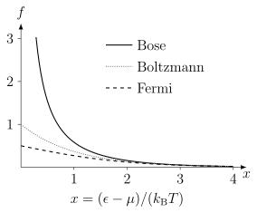
At the same $x=\beta(\epsilon-\mu)>0$, Bose occupation lies above $e^{-x}$ and Fermi occupation below it. All become close for large $x$. The Bose curve diverges as $x\to0^+$; the Fermi curve reaches $1/2$ there and continues toward one for negative $x$, outside the shared domain shown.

Dilute occupations and the classical limit

When $y_i\ll1$,

$$f_\eta=y_i+\eta y_i^2+O(y_i^3).$$

At $y=0.1$, the Bose, Boltzmann, and Fermi means are approximately $0.111$, $0.100$, and $0.0909$. The relative error of the Boltzmann mean, measured against the exact mean, is $y=10\%$ in either case. The comparison holds at fixed activity; fixing density instead requires adjusting $\mu$.

For a uniform free massive gas with equally populated internal components,

$$\mathcal D=\frac{n\lambda_T^d}{g}\ll1,\qquad \lambda_T=\sqrt{\frac{2\pi\hbar^2}{mk_{\mathrm B}T}}$$

is the familiar criterion. Here $g$ counts the degenerate internal modes, and $n$ is total density. Temperature alone is insufficient: mass, density, dimension, and internal populations matter. A trap can have dilute wings and a degenerate center.

The classical grand-canonical description uses a Poisson mode law, $p(n)=e^{-y}y^n/n!$. Bose and Fermi probabilities approach it in absolute differences as $y\to0$, but normalized rare-coincidence correlations can retain order-one exchange signatures. In particular, thermal bosonic bunching does not disappear merely because its count rate becomes small. The classical-limit derivation develops the controlled corrections and explains why $1/N!$ remains in the canonical state count.

High occupation of bosonic modes is a different classical approximation. For a nonconserved oscillator excitation, $\mu=0$ and

$$f_{\mathrm B}=\frac1{e^{\beta\hbar\omega}-1} \simeq\frac{k_{\mathrm B}T}{\hbar\omega} \quad(k_{\mathrm B}T\gg\hbar\omega).$$

This is the large-occupation equipartition or classical-field limit, whereas Maxwell–Boltzmann statistics requires small occupation.

Occupation, uncertainty, and measurement

A thermal bosonic mode has variance larger than its mean. A coherent bosonic state has equal variance and mean; a number state has zero number variance. Bosonic identity therefore does not imply thermal bunching in every preparation. The state and the measured correlation matter.

For a single complete fermionic mode, $n_i^2=n_i$ gives $\operatorname{Var}(n_i)=f_i(1-f_i)$ in any state. Thermal equilibrium determines the particular Fermi–Dirac value of $f_i$; the variance identity itself is kinematic. A detector that combines modes can also measure correlations between their occupations.

Independent ideal modes have zero cross covariance in the grand-canonical ensemble. In a fixed-number state,

$$0=\operatorname{Var}\!\left(\sum_i n_i\right) =\sum_i\operatorname{Var}(n_i)+2\sum_{i<j}\operatorname{Cov}(n_i,n_j).$$

Unless every occupation is sharp, nonzero covariances must cancel the individual variances. Fixed-number conditioning changes the joint distribution even without interactions. Ensemble equivalence explains how local agreement can coexist with different global fluctuations.

From modes to a gas

Occupations weight the spectrum supplied by the Hamiltonian:

$$\overline N=\sum_i f_i,\qquad U=\sum_i\epsilon_i f_i.$$

For a dense spectrum, replace sums by integrals over the density of complete modes $\nu(\epsilon)$, which has units of inverse energy:

$$\overline N\simeq\int d\epsilon\,\nu(\epsilon)f_\eta(\epsilon),\qquad U\simeq\int d\epsilon\,\nu(\epsilon)\epsilon f_\eta(\epsilon).$$

An internal degeneracy already included in $\nu$ must not be counted again. For a continuum dispersion $\epsilon\propto p^s$, the density of states scales as $\epsilon^{d/s-1}$ near the band bottom. A harmonic trap or lattice changes that counting and therefore changes thermodynamics without changing the ideal mode law.

The grand potential $\Omega=-k_{\mathrm B}T\ln\Xi$ gives $P=-(\partial_V\Omega)_{T,\mu}$. In a homogeneous extensive bulk limit, $\Omega=-PV$. Bose exchange lowers the dilute pressure at fixed density and temperature, and Fermi exchange raises it; these effects do not represent new interparticle forces.

For independent thermal modes their von Neumann entropies add:

$$\frac{S}{k_{\mathrm B}}=\sum_i\left[\eta(1+\eta f_i)\ln(1+\eta f_i)-f_i\ln f_i\right].$$

For fermions use $0\ln0=0$ at empty or full occupation. For correlated modes, a sum of individual entropies generally exceeds the joint entropy; independence is part of this formula.

Low-temperature Bose and Fermi behavior

An ideal bosonic ground mode is normalizable only for $\mu<\epsilon_0$ at positive temperature. Its occupation grows as $N_0\simeq[k_{\mathrm B}T] /(\epsilon_0-\mu)$ when the gap to $\mu$ is small. Writing $\mu=\epsilon_0$ directly in a finite-mode grand sum makes it divergent. A Bose-condensed phase instead requires a thermodynamic limit with macroscopic ground-mode occupation and a separately treated condensate. The excited-state density of states determines whether it can saturate.

For fermions at zero temperature, modes below $\mu$ are filled and those above are empty. In a regular bulk gas $\mu$ tends to the Fermi energy. At small nonzero temperature only a shell of width of order $k_{\mathrm B}T$ around $\mu$ changes occupation appreciably. This shell controls the low-temperature heat capacity. Filling successive momentum modes produces degeneracy pressure even without a repulsive potential. The full equations of state are developed for the ideal Bose gas and ideal Fermi gas.

Chemical potential follows the conserved quantity, not simply the exchange sign. Photons and phonons in ordinary equilibrium have $\mu=0$ because their number can change. Separately conserved species can have separate chemical potentials; conversion reactions impose relations among them.

Interactions and observed distributions

An interacting bare-particle Hamiltonian need not factorize into modes. Its equilibrium state still has Gibbs form, but inserting bare energies into an ideal occupation formula is generally incorrect. A controlled quadratic or quasiparticle approximation may restore simple Bose or Fermi factors. Even then, measured bare-particle distributions can contain coherence factors and incoherent spectral weight. In a paired system, diagonalize the appropriate grand Hamiltonian: quasiparticle energies already incorporate its chemical-potential dependence, so subtracting $\mu$ again would count it twice.

Momentum imaging, spectroscopy, noise correlations, and thermodynamic measurements probe different aspects of the state. Detector resolution, interactions, and preparation affect them. Fitting one occupation curve does not establish global thermal equilibrium; agreement with other observables and conserved quantities provides a stronger test.

Exercises

Complete mode labels

A spatial orbital of energy $\epsilon$ is sixfold degenerate because of spin and valley labels: $\sigma=\uparrow,\downarrow$ and $v=1,2,3$. How many identical fermions can occupy the energy level? What is its mean occupation in grand-canonical equilibrium?

Solution

The complete modes are

$$i = (\phi,\sigma,v).$$

There are

$$g = 2\times3 = 6$$

orthogonal modes. Each can contain at most one identical fermion, so the level can contain at most six.

Every mode has mean occupation

$$f_{\mathrm F}(\epsilon) = \frac{1}{e^{\beta(\epsilon-\mu)}+1}.$$

Therefore

$$\overline N_{\epsilon} = 6 f_{\mathrm F}(\epsilon).$$

The exclusion principle is obeyed mode by mode; degeneracy supplies more modes rather than allowing multiple occupancy of one mode.

Zero-temperature Fermi step

Evaluate

$$\lim_{\beta\to\infty} \frac{1}{e^{\beta(\epsilon-\mu)}+1}$$

for $\epsilon<\mu$ and $\epsilon>\mu$. What is the value exactly at $\epsilon=\mu$ for finite $T$?

Solution

If $\epsilon<\mu$, then

$$\beta(\epsilon-\mu) \longrightarrow -\infty,$$

so the exponential vanishes and

$$f_{\mathrm F} \longrightarrow 1.$$

If $\epsilon>\mu$, the exponential diverges and

$$f_{\mathrm F} \longrightarrow 0.$$

At $\epsilon=\mu$ and any finite $T$,

$$f_{\mathrm F}(\mu) = \frac{1}{2}.$$

The value at a single energy does not affect continuum thermodynamic integrals. At zero temperature the distribution is represented by the step function $\Theta(\mu-\epsilon)$ up to that conventional boundary value.

Exchange sector versus observed number variance

Classify the following statements as valid or invalid, and explain: (a) every bosonic state has $\operatorname{Var}(n)>\langle n\rangle$; (b) a Poissonian count distribution proves that particles are distinguishable; (c) a thermal ideal fermionic mode has sub-Poissonian occupation fluctuations.

Solution

(a) is invalid. The formula

$$\operatorname{Var}(n) = f(1+f)$$

describes a thermal ideal bosonic mode. A coherent state has $\operatorname{Var}(n)=\langle n\rangle$, while a number state has zero number variance.

(b) is invalid. Bosonic coherent states are Poissonian, and dilute bosons or fermions approach Poissonian Maxwell–Boltzmann mode statistics. Exchange identity is not erased by a Poissonian observation.

(c) is valid under its stated assumptions because

$$\operatorname{Var}(n) = f(1-f) \leq f.$$

For a single fermionic mode, $n^2=n$ makes this variance identity true in any state; thermal equilibrium is needed to fix its mean by the Fermi–Dirac law. Mode groups and other observables have different counting statistics.

References

• N. W. Ashcroft and N. D. Mermin, Solid State Physics, Brooks/Cole (1976).
• S. N. Bose, “Plancks Gesetz und Lichtquantenhypothese,” Zeitschrift für Physik 26, 178–181 (1924), doi:10.1007/BF01327326.
• P. A. M. Dirac, “On the Theory of Quantum Mechanics,” Proceedings of the Royal Society A 112, 661–677 (1926), doi:10.1098/rspa.1926.0133.
• A. Einstein, “Quantentheorie des einatomigen idealen Gases,” Sitzungsberichte der Preußischen Akademie der Wissenschaften, Physikalisch-mathematische Klasse, 261–267 (1924); “Zweite Abhandlung,” 3–14 (1925).
• E. Fermi, “Zur Quantelung des idealen einatomigen Gases,” Zeitschrift für Physik 36, 902–912 (1926), doi:10.1007/BF01400221.
• A. L. Fetter and J. D. Walecka, Quantum Theory of Many-Particle Systems, Dover (2003).
• K. Huang, Statistical Mechanics, 2nd ed., Wiley (1987).
• M. Kardar, Statistical Physics of Particles, Cambridge University Press (2007).
• L. D. Landau and E. M. Lifshitz, Statistical Physics, Part 1, 3rd ed., Butterworth–Heinemann (1980).
• R. K. Pathria and P. D. Beale, Statistical Mechanics, 3rd ed., Elsevier (2011).
• C. J. Pethick and H. Smith, Bose–Einstein Condensation in Dilute Gases, 2nd ed., Cambridge University Press (2008).