Plasmons in Materials

A material plasmon is a collective charge mode of a specified electronic system and its electromagnetic surroundings. Its energy is not a property of carrier density alone: bands set the current response, surrounding matter sets the electric-field energy, and boundaries select the permitted mode. A probe may couple strongly to one branch and barely at all to another.

This page applies the general theory to bulk solids, conducting sheets, coupled layers and small particles. The examples separate changes of electronic inertia from changes of environment or shape, and distinguish a mode’s existence from its visibility. The hydrodynamic and RPA derivations remain with Plasmons Preview; microscopic dielectric inversion and loss normalization remain with Dielectric Response, Screening, and Loss.

Required background. Plasmons Preview supplies dimensional limits, complex poles, continua and spectral-weight constraints.

Helpful background. Band Theory Overview supplies bands and filling; Drude Theory supplies inertial current response and its relaxation approximation. Random Phase Approximation distinguishes the polarization input from the screened answer, and Particle–Hole Excitations supplies continuum kinematics. Dielectric Response supplies the microscopic-to-macroscopic and probe distinctions used below.

Band currents and the plasma scale

The material phase, carrier populations and occupied bands determine the current response. The benchmarks below have no applied magnetic field. In a collisionless frequency window, define the symmetric longitudinal Drude-weight tensor by

$$\sigma_{ij}(\omega)\simeq \frac{i\mathcal D_{ij}}{\pi(\omega+i0^+)}.$$

This fixes the factor of $\pi$. A three-dimensional conductivity and a sheet conductivity have different units, so their Drude weights must not be exchanged. A collisionless window requires scattering to be slow on the oscillation time scale; it need not extend through interband transitions or polar lattice resonances. Time dependence is $e^{-i\omega t}$.

For one parabolic carrier pocket with density $n$ and positive inertial mass tensor $M$, the elementary intraband result is $\mathcal D=\pi ne^2M^{-1}$, where $e>0$. Contributions of independent electron and hole pockets add with charge squared. Their Hall signals need not add with the same sign. In a nonparabolic or interacting solid, use the appropriate current response rather than replacing $M$ by a density-of-states mass or one measured quasiparticle mass. Optical Conductivity gives the corresponding spectral-weight accounting.

For an isotropic, frequency-independent background relative permittivity $\epsilon_b$, the electrostatic long-wavelength bulk longitudinal benchmark is

$$\Omega_L^2(\widehat{\mathbf q})= \frac{\widehat{\mathbf q}\cdot\mathcal D_{3D} \cdot\widehat{\mathbf q}}{\pi\epsilon_0\epsilon_b}.$$

Here $\epsilon_0$ is the vacuum permittivity. For an isotropic parabolic band, it is useful to distinguish the unscreened Drude scale $\omega_D^2=ne^2/(\epsilon_0m)$ from the background-screened scale $\Omega_L=\omega_D/\sqrt{\epsilon_b}$. A reported “plasma frequency” is incomplete without this distinction.

The background represents degrees of freedom already integrated out. If their resonances lie near the candidate mode, replace a constant $\epsilon_b$ by their causal frequency-dependent response and solve the combined problem. In a polar semiconductor, including the ionic static permittivity and then adding the same LO-phonon oscillator explicitly counts that polarization twice. In a multiband metal, a frequency-dependent interband background can shift a loss maximum substantially without a proportional change in carrier density.

The same warning applies to total electron counts. A low-energy intraband mode uses the relevant current-carrying sector. The complete optical sum over all electrons and transitions is a different constraint; a truncated band model does not inherit it with an arbitrary effective mass. Giuliani and Vignale develop the relation between current response, collective modes and those spectral constraints.

Geometry determines the electric restoring force

A sheet between dielectric half-spaces

For an infinitesimally thin conducting sheet between two local isotropic dielectrics, define $\epsilon_{\rm eff}=(\epsilon_1+\epsilon_2)/2$. In the nonretarded, long-wavelength collisionless limit, the generic sheet result becomes

$$\Omega^2(q,\widehat{\mathbf q})= \frac{q\,\widehat{\mathbf q}\cdot\mathcal D_{2D} \cdot\widehat{\mathbf q}} {2\pi\epsilon_0\epsilon_{\rm eff}}.$$

Thus a directional dispersion measures a combination of current stiffness and environmental screening. It does not independently determine both. For an elliptical parabolic band, $M=\operatorname{diag}(m_x,m_y)$, propagation at angle $\theta$ samples $m_x^{-1}\cos^2\theta+m_y^{-1}\sin^2\theta$. Rotating the momentum and changing the substrate are different experimental controls.

The dielectric average assumes two semi-infinite media with no relevant nearby resonances. Finite layer thickness, anisotropic substrates and multilayer stacks require the corresponding electrostatic Green function. A bulk dielectric function extracted from a periodically repeated slab also contains an arbitrary vacuum-volume normalization unless converted to a sheet response. The material geometry must survive that conversion.

For a doped Dirac band, the useful input is its sheet Drude weight, including the declared degeneracies, filling and temperature. A constant parabolic mass is unnecessary. A $\sqrt q$ dispersion therefore does not, by itself, distinguish a parabolic two-dimensional gas from a Dirac material. The generic density-scaling comparison is developed in Plasmons Preview.

Gates, surfaces and retardation

A perfect metallic plane a distance $d$ from a sheet in a homogeneous dielectric multiplies the nonretarded Coulomb kernel by $1-e^{-2qd}$. At $qd\ll1$, the inertial-response approximation predicts an acoustic branch. Its estimated speed is reliable only when the mode phase velocity is large compared with the relevant electronic velocities, so that the high-frequency polarization expansion applies. Decreasing $q$ alone does not improve this ratio for an acoustic mode; otherwise use the full dynamical polarization. This describes a specified image-charge boundary problem, not a general law for every metal–spacer–sheet stack. Gate conductivity, finite thickness and nonlocal screening can matter when the fields are strongly confined. Alonso-González and collaborators demonstrate acoustic graphene plasmons in a particular gated device and measurement geometry.

At a planar interface between two local isotropic media, the electrostatic surface condition is $\epsilon_m+\epsilon_d=0$. The retarded transverse-magnetic surface mode instead obeys

$$q^2=\frac{\omega^2}{c^2} \frac{\epsilon_m(\omega)\epsilon_d(\omega)} {\epsilon_m(\omega)+\epsilon_d(\omega)},$$

with the transverse wave-vector branches chosen to satisfy the physical decay or outgoing-wave conditions. The algebraic expression alone does not select a bound mode. It assumes semi-infinite media and no additional conducting interface sheet. Finite films and layered structures require their own boundary determinant. Pitarke and collaborators develop these geometry-dependent surface responses.

Use the electrostatic approximation only when the relevant in-plane momentum is well beyond the applicable light-line scales. At fixed real frequency, a propagation experiment commonly determines complex $q$; at fixed real $q$, a temporal response determines complex $\omega$. A spatial decay length and a temporal lifetime are not interchangeable without a dispersion model and a stated amplitude-versus-intensity convention.

Shape shifts a localized resonance

Even with an isotropic material permittivity, different particle axes can resonate at different energies. For a small ellipsoid of volume $V$ in a uniform dielectric, the electrostatic polarizability along principal axis $j$ is

$$\begin{aligned} \alpha_j&=\epsilon_0\epsilon_d V \frac{\epsilon_m-\epsilon_d} {\epsilon_d+L_j(\epsilon_m-\epsilon_d)}, \\ \sum_jL_j&=1. \end{aligned}$$

The positive depolarization factors $L_j$ encode shape. In a lossless local Drude reduction,

$$\begin{aligned} \epsilon_m(\omega)&=\epsilon_\infty- \frac{\omega_D^2}{(\omega+i0^+)^2},\\ \Omega_j^2&=\frac{\omega_D^2} {\epsilon_\infty+(1-L_j)\epsilon_d/L_j}. \end{aligned}$$

The familiar sphere has $L_j=1/3$. A resonance shift caused by changing $L_j$ is not a carrier-density change. This benchmark requires a particle small compared with the relevant electromagnetic wavelengths, a local continuum dielectric description and a uniform surrounding medium. Surface scattering, radiation, nonlocal charge response, spill-out and atomistic structure can change both pole and line shape. A lossless polarizability pole is a reference for those corrections, not a complete extinction spectrum.

A mode and its measured weight

In a crystal, microscopic reciprocal components, layers or orbitals can mix. Find a causal mode of the appropriate dielectric or response matrix and examine its induced charge pattern. For a bulk longitudinal problem a vanishing dielectric eigenvalue can identify a candidate pole of the inverse response. A surface polariton must instead satisfy the electromagnetic boundary problem. Removing denominators to obtain a polynomial can introduce canceled roots; these must be checked in the original response.

A mode couples to a probe through the probe’s spatial profile and operator. In a schematic matrix response $R$, the measured channel involves a contraction such as $g^\dagger Rg$, together with the actual kinematic and detector factors. A pole in $R$ can have zero residue in that contraction. The vector $g$ may depend on momentum, frequency, beam trajectory, polarization or tip height.

For damped modes, right and left eigenvectors need not be conjugate copies. Residues involve both and the frequency derivative of the response kernel. A Euclidean squared component of a dielectric eigenvector is therefore not generally a measured oscillator strength or a probability that the excitation is “electronic.” Dielectric Response supplies the inverse-head and local-field distinctions; the calculations below retain explicit probe weights instead of assigning every determinant zero equal brightness.

Two conducting layers

Consider two identical parabolic sheets of density $n_{2D}$ and mass $m$, separated by $d$ in one homogeneous dielectric $\epsilon$. Neglect tunneling, retardation and dissipation. At momenta where the inertial density response is adequate, let

$$\begin{aligned} \Omega_0^2&=\frac{n_{2D}e^2q}{2m\epsilon_0\epsilon},\\ r&=e^{-qd},\qquad u_\pm=\frac{1}{\sqrt2}\begin{pmatrix}1\\\pm1\end{pmatrix}. \end{aligned}$$

The electrostatic matrix with diagonal entries 1 and off-diagonal entries $r$ gives

$$\Omega_\pm^2=\Omega_0^2(1\pm r).$$

These are in-phase and out-of-phase number-density oscillations of equal-charge sheets. The lower branch is acoustic as $qd\to0$, while both approach independent-sheet modes at large separation for fixed $q$. For the lower acoustic branch, the condition $\Omega_-/(qv_F)\gg1$ is an additional requirement for this inertial estimate; it does not follow merely from $q\to0$. Its sharpness must also be checked against each layer’s particle–hole continuum and other decay channels.

Use a positive potential-energy source $H'=+\sum_l\int d^2r\,U_l n_l$ and define $\delta n=\Pi^R U$. Its retarded density commutator has the $-i/\hbar$ sign, so $\Pi^R$ is the negative of the susceptibility for the source $-f n$ used in Conventions. For a layer profile $U=U_0g$, the projected response in this symmetric model is

$$\begin{aligned} \Pi_g(q,\omega)&=C_q\sum_{s=\pm} \frac{|g^\dagger u_s|^2} {(\omega+i0^+)^2-\Omega_s^2},\\ C_q&=\frac{n_{2D}q^2}{m}. \end{aligned}$$

The positive-frequency area in $-\operatorname{Im}\Pi_g$ is proportional to $|g^\dagger u_s|^2/\Omega_s$. Equal layer amplitudes $g=(1,1)$ make the out-of-phase branch dark even at nonzero in-plane momentum. A one-layer source or a decaying near field need not. A dark mode is not absent, and unequal measured peak areas do not directly give unequal numbers of excitations. A real EELS or optical signal requires its own vertex; this projected density response is an explicit model comparison.

A polar lattice and mobile carriers

A material-specific hybridization model can be built without introducing an arbitrary constant avoided-crossing parameter. Consider an isotropic polar host with one infrared-active oscillator, electronic relative permittivity $\epsilon_\infty$, transverse and longitudinal energies $E_{\rm TO}<E_{\rm LO}$, and dilute parabolic carriers. Set $E=\hbar\omega$ and define the bare electronically screened carrier scale $P=\hbar\omega_D/\sqrt{\epsilon_\infty}$. In the lossless, local, long-wavelength reduction,

$$\frac{\epsilon(E)}{\epsilon_\infty} =\frac{(E+i0^+)^2-E_{\rm LO}^2} {(E+i0^+)^2-E_{\rm TO}^2} -\frac{P^2}{(E+i0^+)^2}.$$

The oscillator already supplies ionic polarization; no ionic static background is added to $P$. This model omits nonlocal carrier pressure, multiple phonon branches, interband structure and damping. It supplies a controlled algebraic benchmark once those omissions are appropriate, not a universal fit to polar solids. The GaAs observation of Mooradian and Wright is an experimental example of carrier–LO-phonon coupling, not evidence that these numerical parameters describe GaAs.

With $x_\pm=E_\pm^2$, the candidate roots are

$$x_\pm={}\frac{E_{\rm LO}^2+P^2}{2} \pm\frac12\sqrt{(E_{\rm LO}^2+P^2)^2 -4P^2E_{\rm TO}^2}.$$

The inverse response also determines their visibility:

$$\begin{gathered} \frac{1}{\epsilon(E)}=\frac{1}{\epsilon_\infty} \left[1+\sum_{s=\pm} \frac{A_s}{(E+i0^+)^2-x_s}\right],\\ A_s=\frac{x_s(x_s-E_{\rm TO}^2)}{x_s-x_{-s}},\\ A_++A_-=P^2+E_{\rm LO}^2-E_{\rm TO}^2. \end{gathered}$$

For distinct positive roots in this passive lossless model, $A_s\ge0$. The integrated loss peak has area $\pi A_s/(2\epsilon_\infty E_s)$, whereas its contribution to $\int_0^\infty E[-\operatorname{Im}\epsilon^{-1}(E)]\,dE$ is $\pi A_s/(2\epsilon_\infty)$. These are different weights. The last identity is this reduced model’s high-frequency moment, not the full electronic sum over omitted material transitions.

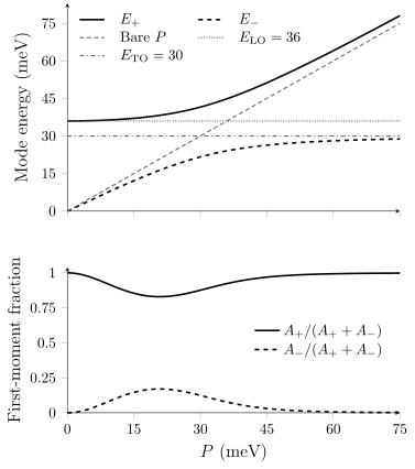
Lossless one-oscillator benchmark with $E_{\rm TO}=30$ and $E_{\rm LO}=36$ meV. The lower panel divides each inverse-dielectric loss first-moment weight by their sum. These fractions describe this response channel, not phonon or electron probabilities. At zero carrier density the lower polynomial root cancels from the response.

As $P\to0$, the upper branch becomes the host LO mode and the lower root loses its residue. If the oscillator strength vanishes, $E_{\rm LO}=E_{\rm TO}$, the apparent phonon factor cancels and only the carrier dielectric pole remains. At coincident roots, take the limit of the original rational response rather than inserting zero denominators into a partial-fraction formula.

For experimental hybridization, follow poles, linewidths, spatial charge and displacement patterns, and the appropriate response residues as carrier density changes. Damping can merge real-frequency maxima even when complex poles remain distinct. Conversely, two fitted peaks are not by themselves proof of two coherently coupled modes. Raman, infrared and electron-loss measurements weight the same coupled system differently.

Interpreting a measured charge mode

Electronic and electrostatic errors enter differently. In a repeated-slab calculation, vacuum spacing and the Coulomb kernel can introduce coupling to unwanted image layers. In a band calculation, momentum sampling and empty-state truncation can change the allowed particle–hole continuum. Converging one does not fix the other. A mode outside the one-pair continuum can still decay through phonons, disorder, multipair processes or radiation; numerical broadening predicts none of those rates.

The measurement also selects a response. Transmission EELS can mix bulk, surface and multiple-scattering losses. Reflection EELS and near fields emphasize boundaries and sample a range of momenta. Nonresonant inelastic x-ray scattering probes a density structure factor. Far-field light has limited in-plane momentum, so patterning, a prism or a tip may be needed to excite a bound surface mode. García de Abajo (2010) develops these trajectory and boundary effects.

Changes with density, propagation direction, dielectric surroundings, layer separation or shape help distinguish competing interpretations. In a near-field fringe experiment, a reflected round trip accumulates twice the propagation phase of a one-way path; the same fringe period then implies a different wave vector. Dispersion, response weight and linewidth together constrain a model more strongly than a single shifted peak. Device performance additionally depends on coupling, dissipation and geometry, which a lossless dispersion alone does not determine.

Exercises

1. Anisotropy or dielectric environment?

A parabolic sheet has $n_{2D}=10^{12}\,\mathrm{cm^{-2}}$, $m_x=0.20m_e$ and $m_y=0.80m_e$. It lies between nondispersive dielectrics with $\epsilon_1=1$ and $\epsilon_2=9$. Use $q=10^6\,\mathrm{m^{-1}}$ and the collisionless electrostatic model at low temperature. Find the two principal-direction plasmon energies and their ratio. Change only $\epsilon_2$ to 3. What mass would a fit infer if it incorrectly retained the original dielectric environment? For a spin-degenerate single-valley band and a 5 nm sheet thickness, check the momentum, inertial-response and electrostatic scale separations.

Solution

The original effective permittivity is 5. Converting the density to $10^{16}\,\mathrm{m^{-2}}$ gives

$$\begin{aligned} \hbar\Omega_x&\simeq2.6257\,\mathrm{meV},\\ \hbar\Omega_y&\simeq1.3128\,\mathrm{meV},\\ \Omega_x/\Omega_y&=2. \end{aligned}$$

With $\epsilon_2=3$, the effective permittivity is 2. Both energies increase by $\sqrt{5/2}$ while their ratio stays 2. The stiffness tensor and carrier population have not changed.

Since $\Omega^2\propto1/(m\epsilon_{\rm eff})$, a fit using the old value 5 would return $m_{\rm fit}=(2/5)m$. It would report $0.08m_e$ and $0.32m_e$ rather than the true masses. The example assumes the substrate change leaves bands, density and scattering unchanged; that assumption must be checked in a real device.

The stated degeneracy gives $E_F=\pi\hbar^2n_{2D}/\sqrt{m_xm_y}\simeq5.9847$ meV, so the degenerate reduction requires $k_{\rm B}T\ll E_F$. Along the light-mass axis, $q/k_{Fx}\simeq0.00564$ and $\Omega_x/(qv_{Fx})\simeq38.88$; the latter ratio is the same along the other principal axis. The transverse-thickness parameter is $qw=0.005$. For the original surrounding media, even the more restrictive light line gives $qc/(\sqrt{\epsilon_2}\Omega_x)\simeq25.05$. These estimates support the long-wavelength inertial and nonretarded reductions for this hypothetical model. They do not check impurity or phonon scattering, which must separately be small compared with the mode frequency.

2. A bilayer branch that disappears from one probe

Take two identical isotropic sheets with $m=0.20m_e$, the density and momentum of Exercise 1, homogeneous $\epsilon=5$, and separation $d=200$ nm. Find the two energies. Compare their positive-frequency integrated density-response areas for $g=(1,1)$, $g=(1,0)$ and the evanescent profile $g=(1,e^{-qd})$. Use the same source normalization within each comparison. Does a weak lower peak imply a missing collective mode?

Solution

Here $qd=0.2$ and $r=e^{-0.2}$. The energies are

$$\begin{aligned} \hbar\Omega_+&=\hbar\Omega_0\sqrt{1+r} \simeq3.54100\,\mathrm{meV},\\ \hbar\Omega_-&=\hbar\Omega_0\sqrt{1-r} \simeq1.11790\,\mathrm{meV}. \end{aligned}$$

Their ratio is

$$\frac{\Omega_+}{\Omega_-} =\sqrt{\frac{1+r}{1-r}}\simeq3.1675.$$

For $g=(1,1)$, the squared overlaps are 2 and 0: only the upper branch appears. For a one-layer source, they are both $1/2$, but the integrated peak areas differ because each includes $1/\Omega_s$. Thus the lower-to-upper area ratio is $\Omega_+/\Omega_-\simeq3.1675$.

For the evanescent source, the squared overlaps are $(1\pm r)^2/2$, and the lower-to-upper area ratio is

$$\begin{aligned} \frac{I_-}{I_+} &=\left(\frac{1-r}{1+r}\right)^{3/2}\\ &=\tanh^{3/2}(0.1)\simeq0.03147. \end{aligned}$$

The same two eigenmodes can therefore produce an absent, dominant or weak lower peak as the source profile changes. These are areas in the specified projected density response, not general EELS count ratios. Finite damping, inequivalent layers and tunneling require a revised response matrix and can change both roots and selection rules.

3. Two hybrid energies and two different spectral weights

Use the polar-host model with $E_{\rm TO}=30$ meV, $E_{\rm LO}=36$ meV and $P=30$ meV. Calculate $E_\pm$, $A_\pm$ and each branch’s fraction of the inverse-dielectric loss first moment. Write the ratio of integrated loss areas. Explain what happens to the apparent two-root description at zero carrier density and at zero oscillator strength.

Solution

The sum and product of the squared energies are

$$\begin{aligned} x_++x_-&=2196\,\mathrm{meV^2},\\ x_+x_-&=810000\,\mathrm{meV^4}. \end{aligned}$$

Solving and substituting the roots into $A_s=x_s(x_s-900)/(x_s-x_{-s})$, with squared energies in $\mathrm{meV^2}$, gives

$$\begin{aligned} E_-&=21.65709\,\mathrm{meV},\\ E_+&=41.55684\,\mathrm{meV},\\ A_-&=160.68945\,\mathrm{meV^2},\\ A_+&=1135.31055\,\mathrm{meV^2}. \end{aligned}$$

The residues sum to $1296\,\mathrm{meV^2}$. The first-moment fractions are $A_s/1296$: 0.123989 for the lower branch and 0.876011 for the upper. The integrated loss-area ratio is

$$\frac{I_-}{I_+}=\frac{A_-E_+}{A_+E_-}.$$

This gives a lower-branch fraction of the total integrated area of 0.213584. The extra frequency factor means that a first-moment fraction is not a peak-area fraction. Neither is an ionic-displacement probability.

At $P=0$, the original dielectric function contains only the polar-host oscillator. The polynomial root at zero cancels from its inverse and has no separate loss weight. If $E_{\rm LO}=E_{\rm TO}$, the oscillator cancels before solving the dielectric equation, leaving the single carrier root $E=P$. At a coincident limiting root, evaluate that original response rather than the singular partial-fraction expression.

4. A shape change misread as a density change

An isotropic Drude ellipsoid has $L_1=0.10$, $L_2=L_3=0.45$, $\epsilon_\infty=4$, $\epsilon_d=2$ and $\hbar\omega_D=1$ eV. Find its three lossless electrostatic resonance energies. If the long-axis resonance is fitted with a spherical model at the same mass and dielectric constants, what ratio $n_{\rm fit}/n$ results? State the main validity conditions for this inference exercise.

Solution

The shape factors sum to one. The pole denominators are 22 along the long axis and $58/9$ along the other axes, so

$$\begin{aligned} \hbar\Omega_1&=\frac{1}{\sqrt{22}}\,\mathrm{eV} \simeq0.21320\,\mathrm{eV},\\ \hbar\Omega_{2,3}&=\frac{3}{\sqrt{58}}\,\mathrm{eV} \simeq0.39392\,\mathrm{eV}. \end{aligned}$$

A sphere has denominator $\epsilon_\infty+2\epsilon_d=8$. Matching its peak to the long-axis energy requires $\omega_{D,\rm fit}^2/8=\omega_D^2/22$. At fixed mass,

$$\frac{n_{\rm fit}}n=\frac{\omega_{D,\rm fit}^2}{\omega_D^2} =\frac4{11}.$$

The true carrier density has not changed. The calculation assumes an electrostatically small particle, local isotropic material response, a homogeneous environment and negligible loss when locating the poles. Radiation, boundary scattering, nonlocality and atomistic size effects are separate checks; the exercise does not establish that a fabricated ellipsoid realizes the ideal model.

References

• P. Alonso-González, A. Y. Nikitin, Y. Gao, A. Woessner, M. B. Lundeberg, A. Principi, N. Forcellini, W. Yan, S. Vélez, A. J. Huber, K. Watanabe, T. Taniguchi, F. Casanova, L. E. Hueso, M. Polini, J. Hone, F. H. L. Koppens and R. Hillenbrand, “Acoustic terahertz graphene plasmons revealed by photocurrent nanoscopy,” Nature Nanotechnology 12, 31–35 (2017), doi:10.1038/nnano.2016.185. A gated-sheet realization and its spatially resolved measurement.
• F. J. García de Abajo, “Optical excitations in electron microscopy,” Reviews of Modern Physics 82, 209–275 (2010), doi:10.1103/RevModPhys.82.209. Electron trajectories, interfaces and the relation between material response and measured losses.
• G. F. Giuliani and G. Vignale, Quantum Theory of the Electron Liquid (Cambridge University Press, 2005). Current response, collective charge modes, continua and spectral constraints.
• A. Mooradian and G. B. Wright, “Observation of the Interaction of Plasmons with Longitudinal Optical Phonons in GaAs,” Physical Review Letters 16, 999–1001 (1966), doi:10.1103/PhysRevLett.16.999. Experimental carrier–lattice hybridization in a specified polar semiconductor.
• J. M. Pitarke, V. M. Silkin, E. V. Chulkov and P. M. Echenique, “Theory of surface plasmons and surface-plasmon polaritons,” Reports on Progress in Physics 70, 1–87 (2007), doi:10.1088/0034-4885/70/1/R01. Surface, interface and localized response with explicit geometry and approximation boundaries.