Excitons in Materials

An exciton is a neutral excitation in which an electron and the hole left in an occupied electronic state are bound to one another. Binding changes the neutral excitation spectrum: a bound state lies below the corresponding unbound electron–hole continuum. It does not follow that this state is the lowest excitation of the material, that it can absorb a photon in a given geometry, or that a population of such states forms a condensate.

This page develops the bound-pair problem and the tests that connect it to material spectra. The detailed comparison among charge, quasiparticle, optical and transport gaps remains in Band Gaps. Here the emphasis is on the interaction kernel, the pair wavefunction, internal and center-of-mass quantum numbers, and what a measured line can establish.

Required background. Band Theory Overview supplies bands, occupations and the distinction between quasiparticle energies and auxiliary one-electron eigenvalues. Particle–Hole Excitations supplies number-conserving pair states, momentum transfer and the unbound continuum.

Helpful background. Effective Mass supplies the band-edge expansion, and The Hydrogen Atom supplies the Coulomb bound-state problem. Spectral Functions separates energy, weight and linewidth; Dielectric Response supplies screening conventions.

A bound pair below a specified continuum

Start with a clean, undoped semiconductor or insulator at low excitation density. Assume well-defined valence and conduction quasiparticles. The reference has filled valence states and empty conduction states; electron number is unchanged when an electron moves between them. With crystal momentum transfer $\mathbf Q$, write a one-pair approximation to a neutral eigenstate as

$$\lvert S,\mathbf Q\rangle =\sum_{vc\mathbf k} A^S_{vc\mathbf k}(\mathbf Q) a^\dagger_{c,\mathbf k+\mathbf Q}a_{v,\mathbf k} \lvert 0\rangle.$$

$S$ labels the internal state, including whatever spin, valley and band labels the model retains. $\mathbf Q$ is defined modulo a reciprocal-lattice vector. The hole has the opposite momentum to the removed electron; this is why the pair carries $\mathbf Q$, rather than $2\mathbf k+\mathbf Q$.

In the specified pair channel, the separated quasiparticle threshold is

$$E_{\mathrm{cont}}(\mathbf Q) =\min_{vc\mathbf k} \bigl[E^{\mathrm{QP}}_{c,\mathbf k+\mathbf Q} -E^{\mathrm{QP}}_{v,\mathbf k}\bigr].$$

The minimization includes the allowed band and spin sectors, not unrelated transitions. For a discrete state of excitation energy $E_S(\mathbf Q)$, define

$$E_b^S(\mathbf Q) =E_{\mathrm{cont}}(\mathbf Q)-E_S(\mathbf Q)>0.$$

Both energies refer to the same sample environment, charge state, temperature and momentum sector. Subtracting a monolayer optical line from a bulk gap, or from a Kohn–Sham gap without an excitation-energy justification, does not measure binding. For an indirect semiconductor, the fundamental pair minimum can occur at finite $\mathbf Q$ while near-normal optical absorption samples a direct channel near zero in-plane momentum.

This definition permits a state bound against pair dissociation to have a finite lifetime against recombination, phonon-assisted transfer or other decay. A resonance embedded in an allowed continuum requires a resonance description; a broadened absorption maximum alone is insufficient evidence of a discrete bound state. In a strongly correlated material without sharp electron and hole edges, an exact neutral response can still contain a bound excitation, but the independent-quasiparticle threshold above may cease to be a controlled construction.

From a pair kernel to the exciton wavefunction

In a static screened, resonant electron–hole approximation, a Bethe–Salpeter-type equation has the form

$$\begin{aligned} \Delta E_I(\mathbf Q) A_I^S +\sum_J K_{IJ}(\mathbf Q)A_J^S &=E_S(\mathbf Q)A_I^S, \\ I&=(v,c,\mathbf k). \end{aligned}$$

Here $\Delta E_I$ is the quasiparticle energy difference. The kernel $K$ contains an attractive screened direct contribution and electron–hole exchange, with spin factors and matrix elements appropriate to the retained channel. It is not a scalar dielectric constant attached to every matrix element. Normalize $\sum_I|A_I^S|^2=1$ in a finite orthonormal transition basis; Brillouin-zone quadrature weights must be included consistently when taking the continuum limit.

The Hermitian resonant eigenproblem neglects coupling to the antiresonant sector, the Tamm–Dancoff approximation. It also presumes the specified treatment of screening, quasiparticle self-energies and occupied-state factors. Dynamical screening, strong resonant–antiresonant coupling, substantial doping or multipair character require a more general response problem. Onida, Reining and Rubio explain the relation between the one-particle inputs and the two-particle kernel; agreement of a ground-state energy calculation alone does not validate this excitation problem.

The corresponding two-coordinate amplitude is

$$\Psi_{S\mathbf Q}(\mathbf r_e,\mathbf r_h) =\sum_{vc\mathbf k} A^S_{vc\mathbf k}(\mathbf Q) \psi_{c,\mathbf k+\mathbf Q}(\mathbf r_e) \psi^*_{v,\mathbf k}(\mathbf r_h).$$

Fixing the hole position and inspecting the conditional electron distribution distinguishes an extended pair from one concentrated on a molecule, neighboring sites or different layers. An electron–hole separation is an internal length; it is not the distance over which the pair’s center of mass remains coherent. For example, rephasing each Bloch orbital as $\psi_n\to e^{i\theta_n}\psi_n$ changes the transition basis by $e^{i(\theta_c-\theta_v)}$. Its coefficient must change oppositely:

$$A_{vc\mathbf k}^S\longrightarrow e^{i(\theta_{v\mathbf k}-\theta_{c,\mathbf k+\mathbf Q})} A_{vc\mathbf k}^S.$$

The factors cancel in $\Psi$. The individual complex coefficients depend on this basis choice; the conditional density does not.

The Wannier–Mott limit

Suppose a direct gap involves one isotropic parabolic conduction edge of positive mass $m_e^*$ and one valence maximum with positive hole mass $m_h^*$. Neglect exchange and assume a local, frequency-independent attractive potential. Define

$$\begin{gathered} M=m_e^*+m_h^*,\\ \mu^{-1}=(m_e^*)^{-1}+(m_h^*)^{-1},\\ \mathbf r=\mathbf r_e-\mathbf r_h,\\ \mathbf R=\frac{m_e^*\mathbf r_e+m_h^*\mathbf r_h}{M}. \end{gathered}$$

The kinetic energy separates into relative and center-of-mass motion. Expanding the band states around the two extrema and projecting onto their slowly varying envelopes gives

$$\left[-\frac{\hbar^2}{2\mu}\nabla_{\mathbf r}^2 +V(\mathbf r)\right]\phi_\nu =-E_b^\nu\phi_\nu,$$

and

$$\begin{aligned} E_\nu(\mathbf Q) &=E_g^{\mathrm{QP}}-E_b^\nu +\frac{\hbar^2Q^2}{2M},\\ E_{\mathrm{cont}}(\mathbf Q) &=E_g^{\mathrm{QP}}+\frac{\hbar^2Q^2}{2M}. \end{aligned}$$

The continuum has the same center-of-mass kinetic term because its minimum at fixed total momentum occurs at zero relative momentum. Thus a change in $Q$ need not change the binding energy. Anisotropic masses, multiband mixing, exchange and lattice-scale structure can invalidate this simple separation or dispersion.

For a three-dimensional Coulomb model let

$$V(r)=-\frac{C}{r},\qquad C=\frac{e^2}{4\pi\epsilon_0\epsilon_r}.$$

The hydrogenic rescaling gives

$$\begin{gathered} a_X=\frac{\hbar^2}{\mu C},\qquad R_X=\frac{\mu C^2}{2\hbar^2},\\ E_b^n=\frac{R_X}{n^2},\qquad n=1,2,\ldots. \end{gathered}$$

$a_X$ is the Bohr length of this model, not an unspecified experimental “radius”: the 3D ground state has $\langle r\rangle=3a_X/2$. The mass is the reduced mass, not $M$ and not the free-electron mass $m_0$.

Control requires an envelope much larger than a unit cell, momenta narrow enough to sample approximately quadratic bands, a binding scale small enough to avoid omitted bands, and a justified screened potential over the sampled momenta and frequencies. A large radius is necessary for a simple envelope description but does not prove all these conditions. In a polar crystal, inserting the static permittivity by default can double-count or misrepresent lattice polarization: compare the internal electronic motion and phonon scales, or include dynamical screening and exciton–phonon dressing explicitly.

Screening and spatial character in reduced dimensions

Confinement changes both kinetic energy and the electrostatic boundary problem. A strictly two-dimensional particle pair interacting through $-C/r$ has

$$E_b^n=\frac{R_X}{(n-\tfrac12)^2}, \qquad n=1,2,\ldots.$$

Its ground-state binding is $4R_X$. This is a useful analytic benchmark, not a universal formula for an atomically thin semiconductor.

For a polarizable sheet between insulating half spaces, a common long-wavelength static kernel is

$$\begin{gathered} V(q)=-\frac{e^2}{2\epsilon_0\kappa q(1+r_0q)},\\ \kappa=\frac{\epsilon_{\mathrm{top}}+\epsilon_{\mathrm{bottom}}}{2},\\ V(\mathbf r)=\int\frac{d^2q}{(2\pi)^2} e^{i\mathbf q\cdot\mathbf r}V(q). \end{gathered}$$

Here $q=|\mathbf q|$, the two permittivities are relative permittivities of the external media, and $r_0$ is the screening length as it appears in this denominator, including its environmental dependence. Other conventions absorb $\kappa$ into a differently named length. $V(q)$ has units of energy times area.

The potential becomes Coulomb-like at large separation and logarithmic at short separation within the sheet model. Its momentum dependence changes the relative spacings of the exciton levels; fitting one line to a three-dimensional hydrogen spectrum cannot determine a unique gap and dielectric constant. Cudazzo, Tokatly and Rubio derive the nonlocal sheet-screening mechanism. At lattice-scale separation, finite thickness, local fields and orbital structure must replace or qualify the continuum kernel.

Different names identify different parts of the wavefunction:

• Wannier–Mott: a relative envelope extends over many unit cells and a band-edge description is useful.
• Frenkel: the electron–hole excitation is concentrated on an atom or molecular unit. Transfer between units can still produce a dispersive exciton band; small internal size does not imply an immobile center of mass.
• Charge-transfer: the electron and hole occupy different chemical units or orbitals. A localized basis and the corresponding interaction matrix elements often provide a better starting point than one scalar mass.
• Interlayer: electron and hole weight lies mainly in different layers, giving an out-of-plane dipole. A toy uniform-medium potential $-C/\sqrt{r^2+d^2}$ illustrates the softened short-range attraction; a real heterostructure needs its layer-dependent screening and hybridization.
• Moiré: a long-period texture modifies the pair’s center-of-mass energy and possibly its internal composition. If the pair is small compared with the moiré period and internal excitations are well separated, one may project onto an internal state and add a periodic potential to its center-of-mass Hamiltonian. Otherwise coupled internal states and local band alignment matter.

These labels are not mutually exclusive. An interlayer exciton can have a large in-plane Wannier envelope and a center of mass trapped by a moiré potential. Binding energy alone does not fix its spatial class. Transition-Metal Dichalcogenides, Van der Waals Heterostructures and Moiré Superlattices supply the platform-specific setting.

Brightness, spin, valley and center-of-mass momentum

Existence and optical weight are separate questions. In a chosen polarization channel $\mathbf e$, a schematic transition amplitude is

$$\mathcal M_{S,\mathbf e} =\sum_{vc\mathbf k} (A^S_{vc\mathbf k})^*\, \mathbf e\cdot\mathbf d_{cv}(\mathbf k).$$

$\mathbf d_{cv}$ is the consistently defined interband transition matrix element; for example, $\mathbf d_{cv}=\langle c|\mathbf D|v\rangle$ for the chosen dipole operator. It transforms with the same phase as $A$, so $A^*\mathbf d_{cv}$ is unchanged. Overall sample normalization and photon factors belong in the absorption calculation. Different transition components can add or cancel. A bound eigenvalue by itself supplies neither this amplitude nor a measured intensity.

In the simplest direct-gap envelope limit with a nearly constant allowed interband matrix element, the optical weight is proportional to $|\phi_\nu(0)|^2$. The allowed one-photon hydrogenic series therefore selects internal $s$ envelopes in that model. Elliott’s absorption treatment connects the discrete series and the interacting continuum. Crystal symmetry, band mixing, two-photon processes and the operator used to probe the material change the selection rules.

“Dark” must name its restriction. A transition can be spin forbidden, excluded by the polarization or valley selection rule, or outside the available photon momentum. Spin–orbit coupling makes pure spin labels approximate; exchange can split and mix internal states. Disorder, phonons, magnetic fields or a different optical channel may activate a weak transition without changing whether the pair is bound.

For a translationally invariant two-dimensional layer in a uniform optical medium of refractive index $n_r$, direct emission into propagating photons requires

$$Q\lesssim q_\gamma =\frac{n_r E_X}{\hbar c}.$$

This is the approximate light-cone condition, treating the small center-of-mass energy as negligible compared with the optical energy $E_X$. Even an internally allowed exciton at $Q>q_\gamma$ cannot emit directly into that photon continuum while conserving in-plane momentum. Cavities, interfaces, near fields and finite collection angles require their actual electromagnetic modes.

Wang and colleagues discuss how internal selection rules and this momentum restriction jointly determine emission from monolayers. A thermal population occupies many momenta; its observed decay is not generally the lifetime of a single zero-momentum bright state.

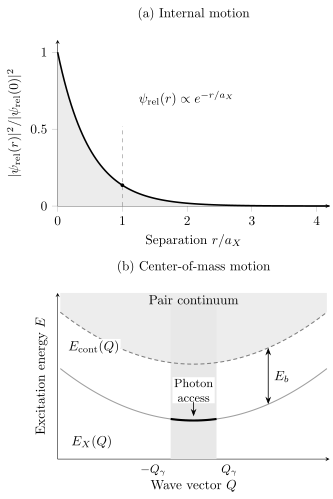
Internal separation and center-of-mass motion describe different coordinates. In (a), an exponential relative envelope fixes an internal length; the ordinate is local density relative to its value at the origin, not a radial probability distribution. In (b), the exciton branch and corresponding free-pair threshold have the same center-of-mass mass in the parabolic benchmark. The shaded photon-access interval is a cut through the two-dimensional light cone and is deliberately exaggerated. Lower-panel energies and momenta are schematic.

Lifetimes and the limits of a dilute exciton gas

Exciton–phonon coupling can transfer momentum between bright and dark sectors, relax internal states, broaden lines or eventually dissociate a pair. Recombination, defect trapping and transfer between layers can remove population. The same measured emission transient can therefore change when relaxation changes, even if the intrinsic radiative matrix element is unchanged.

For an isolated homogeneous optical transition in a Markovian model, distinguish population time $T_1$ from coherence time $T_2$:

$$\frac{1}{T_2}=\frac{1}{2T_1}+\frac{1}{T_\phi}, \qquad \Gamma_E^{\mathrm{FWHM}}=\frac{2\hbar}{T_2}.$$

$T_\phi$ describes pure dephasing and the linewidth formula assumes a Lorentzian homogeneous line. Inhomogeneous broadening, spectral diffusion and coupled reservoirs spoil a direct conversion from an ensemble linewidth or photoluminescence decay to a microscopic lifetime. Pump–Probe Spectroscopy explains how time-resolved signals constrain these processes.

Composite-boson language is most useful when pairs overlap weakly: parametrically $n_Xa_X^d\ll1$ in dimension $d$, with the actual internal size used. It does not remove the fermionic Pauli constraints. Increasing density changes screening and occupations, permits biexcitons or carrier-bound complexes, and can destroy a separated bound-pair description. A density-driven ionization or Mott crossover is not fixed by one universal value of $n_Xa_X^d$.

Likewise, $E_b\gg k_BT$ suppresses thermal dissociation energetically but does not determine the bound fraction without density, entropy, degeneracies and equilibration rates. Exercise 4 makes this distinction quantitative. Optically pumped populations may never reach chemical equilibrium before recombination.

A bound exciton does not establish an excitonic insulator or an exciton condensate. Those claims require an appropriate many-body order or coherence criterion and evidence that excludes competing lattice, charge-transfer or nonequilibrium explanations. A dilute optical resonance, enhanced luminescence or long lifetime is insufficient. Exciton–photon strong coupling produces polaritons, whose dispersion and population dynamics include the photon component.

Identifying an exciton in a material

An absorption or reflectance line is interpreted together with the appropriate electron–hole continuum, optical matrix elements and propagation through the sample. Photoluminescence additionally depends on how the emitting state was populated and relaxed. Polarization, field response, an internal excited-state series or momentum dispersion can help distinguish an exciton from a defect or vibronic transition. No single line shape establishes all these properties.

The calculation has complementary resolution limits. A large-radius exciton is narrow in momentum space, so a coarse momentum mesh can miss its binding even if the band edges look converged. Empty bands, dielectric cutoffs and the transition basis affect the screened kernel. A repeated-layer calculation also needs the intended dielectric environment and control of unwanted image-layer screening. These errors can change the wavefunction and the continuum differently.

Changing the dielectric surroundings can shift both the quasiparticle gap and the binding energy. The shifts may partly cancel in the optical line. A small line shift therefore does not prove weak environmental screening; conversely, a precise optical energy does not remove uncertainty in the continuum needed to infer binding. The two quantities should describe the same sample and channel.

Optical Conductivity develops optical response, Raman and Optical Spectroscopy explains experimental signals, and Electronic Structure Methods Overview distinguishes the required one- and two-particle calculations.

Exercises

1. Binding energy, reduced mass and envelope control

A hypothetical three-dimensional direct-gap semiconductor has $m_e^*=0.20m_0$, $m_h^*=0.30m_0$, $\epsilon_r=12$ and $E_g^{\mathrm{QP}}=2.000\,\mathrm{eV}$. Use the static Coulomb envelope model. Find $M$, $\mu$, the ground-state binding and optical energy if that state is allowed, and $a_X$. Compare the length with a lattice spacing $a=0.50\,\mathrm{nm}$. Does this comparison validate the entire model? Use the free hydrogen values $a_0=0.0529177\,\mathrm{nm}$ and $R_H=13.6057\,\mathrm{eV}$.

Solution

The two masses serve different purposes:

$$M=0.50m_0,\qquad \mu=0.12m_0.$$

Rescaling the Coulomb problem gives

$$\begin{aligned} E_b^{1s}&=R_H\frac{\mu/m_0}{\epsilon_r^2} =11.34\,\mathrm{meV},\\ E_{1s}(0)&=1.98866\,\mathrm{eV},\\ a_X&=a_0\frac{\epsilon_r}{\mu/m_0} =5.292\,\mathrm{nm}. \end{aligned}$$

Thus $a_X/a\simeq10.6$, and the envelope samples a momentum scale $1/a_X\simeq0.189\,\mathrm{nm}^{-1}$, much smaller than $2\pi/a\simeq12.6\,\mathrm{nm}^{-1}$. This supports a slowly varying envelope but does not prove band parabolicity over that range, isolation from other bands, or static local screening. Those need independent material information. Using $M$ in the binding formula would overestimate binding by a factor $0.50/0.12\simeq4.17$.

2. A variational sheet exciton

Use the two-dimensional screened kernel above and the normalized trial envelope

$$\phi_b(r)=\sqrt{\frac{2}{\pi b^2}}e^{-r/b}, \qquad b>0.$$

Find its density form factor and variational energy. Recover the exact two-dimensional Coulomb ground state when $r_0=0$. Explain the direction of the energy and binding bounds for $r_0>0$. As a numerical example, minimize for $\mu=0.20m_0$, $\kappa=4$ and $r_0=4\,\mathrm{nm}$. The useful identity is $\int_0^\infty r e^{-\alpha r}J_0(qr)\,dr=\alpha/(\alpha^2+q^2)^{3/2}$.

Solution

The radial measure $2\pi r\,dr$ gives unit norm. With $C=e^2/(4\pi\epsilon_0\kappa)$, the density form factor and kinetic expectation are

$$\begin{aligned} \rho_b(q)&=\int d^2r\,e^{i\mathbf q\cdot\mathbf r}|\phi_b(r)|^2\\ &=\bigl[1+(qb/2)^2\bigr]^{-3/2},\\ \langle T\rangle_b&=\frac{\hbar^2}{2\mu b^2}. \end{aligned}$$

Using the declared Fourier measure,

$$E_{\mathrm{var}}(b) =\frac{\hbar^2}{2\mu b^2} -C\int_0^\infty \frac{dq}{(1+r_0q)[1+(qb/2)^2]^{3/2}}.$$

For $r_0=0$ the integral is $2/b$. Minimization gives $b=a_X/2$ and $E_{\mathrm{var}}=-4R_X$, where $a_X=\hbar^2/(\mu C)$ and $R_X=\mu C^2/(2\hbar^2)$. This exponential is the exact 2D Coulomb ground state, so equality holds in the variational bound. It is not the 3D hydrogen ground state restricted to a plane with its old eigenvalue retained.

For the numerical parameters, minimization gives $b\simeq2.490\,\mathrm{nm}$ and $E_{\mathrm{var}}\simeq-84.34\,\mathrm{meV}$. The same masses and surroundings with $r_0=0$ would give $b\simeq0.5292\,\mathrm{nm}$ and $E_b\simeq680.3\,\mathrm{meV}$. The large difference illustrates why the sheet polarizability cannot be replaced by the external $\kappa$ alone. These are model benchmarks, not values assigned to a named material.

The Variational Principle gives $E_0\leq\min_b E_{\mathrm{var}}$. If the trial minimum is negative, then $E_b=-E_0\geq-\min_b E_{\mathrm{var}}$: the estimated binding is a lower bound within this kernel, not an upper bound on material binding. Errors in the kernel itself are outside that theorem.

Screening also weakens attraction relative to the same-environment unscreened Coulomb model. Indeed, $1/(1+r_0q)=\int_0^\infty e^{-t}e^{-r_0qt}\,dt$ writes the real-space potential as an average of $-C/\sqrt{r^2+(r_0t)^2}$, each less attractive than $-C/r$. Hence $E_b\leq4R_X$ for this model. Together the two bounds give a useful numerical check.

3. An internally bright population outside the light cone

Consider one internally allowed exciton branch in a uniform two-dimensional layer. Its center-of-mass dispersion is $E_X+\hbar^2Q^2/(2M)$ and its population follows a nondegenerate Boltzmann distribution at temperature $T$. Show that the fraction inside the approximate photon cone is $1-e^{-E_\gamma/(k_BT)}$, where $E_\gamma=\hbar^2q_\gamma^2/(2M)$. Evaluate it for $M=0.80m_0$, $E_X=1.70\,\mathrm{eV}$, $n_r=1.5$ and $T=20\,\mathrm K$, using $\hbar c=197.327\,\mathrm{eV\,nm}$, $\hbar^2/(2m_0)=0.03810\,\mathrm{eV\,nm^2}$ and $k_B=0.08617\,\mathrm{meV/K}$. Can this fraction alone determine a measured luminescence lifetime?

Solution

The two-dimensional momentum measure is $2\pi Q\,dQ$. Its normalized cumulative population gives

$$\begin{aligned} f_\gamma &=\frac{\int_0^{q_\gamma}Qe^{-\beta\hbar^2Q^2/(2M)}\,dQ} {\int_0^\infty Qe^{-\beta\hbar^2Q^2/(2M)}\,dQ}\\ &=1-e^{-\beta E_\gamma}. \end{aligned}$$

The numerical scales are

$$\begin{gathered} q_\gamma\simeq0.01292\,\mathrm{nm}^{-1},\\ E_\gamma\simeq0.00795\,\mathrm{meV},\qquad f_\gamma\simeq0.00460. \end{gathered}$$

Only about $0.46\%$ of this thermal branch is in the cone, even though its internal transition is allowed. If scattering maintains that thermal distribution and the radiative rate were constant inside the cone and zero outside, the population rate would be $f_\gamma\Gamma_0$. That is an additional kinetic model. Real momentum-dependent photon coupling, internal dark branches, nonradiative decay and slow refilling of the cone can change the result. A measured emission lifetime therefore cannot be read from $f_\gamma$ alone.

4. Binding does not fix the ionized fraction

Consider a dilute, equilibrated two-dimensional mixture of free electrons, free holes and one internal exciton species, all with parabolic dispersions. Let the degeneracies be $g_e,g_h,g_X$, the binding be $E_b>0$, and $M=m_e^*+m_h^*$. Take each species to be a classical ideal gas and set the free electron and hole band-edge energies to zero, so the exciton internal energy is $-E_b$. Derive the mass-action relation. With charge neutrality $n_e=n_h=x$ and total pair density $n_p=x+n_X$, show why even a large fixed $E_b/k_BT$ cannot determine $x/n_p$.

Solution

The two-dimensional ideal-gas densities are

$$\begin{aligned} n_e&=g_e\frac{m_e^*k_BT}{2\pi\hbar^2}e^{\beta\mu_e},\\ n_h&=g_h\frac{m_h^*k_BT}{2\pi\hbar^2}e^{\beta\mu_h},\\ n_X&=g_X\frac{Mk_BT}{2\pi\hbar^2}e^{\beta(\mu_X+E_b)}. \end{aligned}$$

Chemical equilibrium of $e+h\rightleftharpoons X$ requires $\mu_X=\mu_e+\mu_h$. Eliminating the chemical potentials gives

$$\frac{n_en_h}{n_X} =\frac{g_eg_h}{g_X} \frac{\mu k_BT}{2\pi\hbar^2} e^{-E_b/(k_BT)} \equiv K(T).$$

$K$ has units of inverse area. Charge neutrality gives $x^2=K(n_p-x)$; with $y=x/n_p$,

$$\frac{y^2}{1-y}=\frac{K}{n_p}.$$

At fixed $T$ and $E_b$, $n_p\ll K$ gives $y\simeq1-n_p/K$, while $n_p\gg K$ gives $y\simeq\sqrt{K/n_p}$, if the ideal-gas and dilute-pair assumptions still hold. The entropy of two free species matters even for a favorable binding energy. For example, $n_p=K$ gives $y=(\sqrt5-1)/2\simeq0.618$, independent of how small $K$ itself is.

Before applying either limit, check $n_i\lambda_i^2/g_i\ll1$, where $\lambda_i^2=2\pi\hbar^2/(m_i k_BT)$, weak pair overlap, negligible additional complexes and equilibration faster than recombination. The ideal-mixture result is not a prediction for a dense pumped semiconductor with changing screening.

References

• P. Cudazzo, I. V. Tokatly and A. Rubio, “Dielectric screening in two-dimensional insulators: Implications for excitonic and impurity states in graphane,” Physical Review B 84, 085406 (2011), doi:10.1103/PhysRevB.84.085406. Derives the nonlocal sheet-screening kernel and its spatial limits.
• R. J. Elliott, “Intensity of Optical Absorption by Excitons,” Physical Review 108, 1384–1389 (1957), doi:10.1103/PhysRev.108.1384. Connects excitonic bound states and continuum enhancement to optical selection.
• G. Onida, L. Reining and A. Rubio, “Electronic excitations: density-functional versus many-body Green’s-function approaches,” Reviews of Modern Physics 74, 601–659 (2002), doi:10.1103/RevModPhys.74.601. Develops the relation between quasiparticle inputs, electron–hole kernels and optical response.
• G. Wang, A. Chernikov, M. M. Glazov, T. F. Heinz, X. Marie, T. Amand and B. Urbaszek, “Colloquium: Excitons in atomically thin transition metal dichalcogenides,” Reviews of Modern Physics 90, 021001 (2018), doi:10.1103/RevModPhys.90.021001. Reviews internal states, exchange, optical selection and exciton relaxation in monolayer semiconductors.