Optical Conductivity

Optical conductivity describes the amplitude and phase of a material’s current at each driving frequency. Its dissipative part measures absorption by that current channel; its reactive part records the out-of-phase response required by causality. A useful interpretation keeps both parts, the zero-frequency weight and the experimental frequency window. A narrow peak, an absorption threshold or a reduction of low-energy weight is not by itself a unique microscopic diagnosis.

Kubo Formula in Materials constructs the intrinsic response from a gauged Hamiltonian, including contact terms and current matrix elements. The discussion below interprets its spectrum. Terahertz and Infrared Probes explains how reflectance, transmission and phase measurements determine that response. A measured transmission dip is not yet a conductivity peak.

Required background. Kubo Formula in Materials supplies the physical response, spectral normalization and optical order of limits.

Helpful background. Drude Theory supplies the relaxation-time benchmark; Band Theory Overview supplies filling and transition states; Sum Rules supplies exact integral constraints; Spectral Functions distinguishes one-particle spectra; Terahertz and Infrared Probes supplies the measurement-to-response conversion.

Complex current response and absorbed power

Use the macroscopic electric field inside a homogeneous material, weak enough for linear response, with time dependence $e^{-i\omega t}$. In the local optical limit,

$$\mathbf j(\omega)=\boldsymbol\sigma(\omega)\mathbf E(\omega).$$

Bulk conductivity has SI units $\mathrm{S\,m^{-1}}$. A two-dimensional sheet instead has a sheet conductance in siemens. The field here is the total field acting on the material, after its electrodynamic boundary problem has been solved; it is not generally the incident field. Spatial dispersion requires $\boldsymbol\sigma(\mathbf Q,\omega)$ and a specified longitudinal or transverse limit. The formulas below do not identify those limits when they differ.

For a scalar or principal-axis channel, write

$$\sigma(\omega)=\sigma_1(\omega)+i\sigma_2(\omega).$$

Real time-domain response gives $\sigma_1(-\omega)=\sigma_1(\omega)$ and $\sigma_2(-\omega)=-\sigma_2(\omega)$. For a harmonic field with complex amplitude $E$, the cycle-averaged power absorbed per volume is $\overline p=\sigma_1|E|^2/2$. A passive equilibrium scalar channel therefore has $\sigma_1(\omega)\ge0$ for $\omega>0$.

For a real drive $E(t)=E_0\cos\omega t$, the current is $j(t)=E_0[\sigma_1\cos\omega t+\sigma_2\sin\omega t]$. The cosine term contributes a positive average of $jE$ in a passive material; the sine term alternately stores and returns energy, with zero average over a cycle. This is the distinction between dissipative and reactive response.

For a tensor, the corresponding statement is

$$\begin{aligned} \overline p&=\frac12\mathbf E^\dagger \boldsymbol\sigma_H\mathbf E,\\ \boldsymbol\sigma_H&=\frac{\boldsymbol\sigma+\boldsymbol\sigma^\dagger}{2} \succeq0. \end{aligned}$$

The Hermitian part must be positive semidefinite. It is not necessary that the real part of every off-diagonal entry be positive. Polarization-dependent absorption is a property of the full quadratic form. The sign of $\sigma_2$ alone does not diagnose gain: capacitive and inductive responses can both be passive.

Causality links the two parts

A retarded conductivity is analytic for $\operatorname{Im}z>0$. Once its high-frequency behavior is controlled, its real and imaginary parts obey Kramers–Kronig relations. A zero-frequency pole needs explicit treatment. Define

$$\begin{aligned} \sigma(z)&=\frac{iD_\delta}{z}+\sigma^{\mathrm{reg}}(z),\\ \sigma_1(\omega)&=\pi D_\delta\delta(\omega) +\sigma_1^{\mathrm{reg}}(\omega). \end{aligned}$$

The notation $D_\delta$ specifies the delta weight in this normalization, without yet assigning its mechanism. For $\omega>0$, with no other necessary subtractions,

$$\sigma_2(\omega)=\frac{D_\delta}{\omega} -\frac{2\omega}{\pi}\operatorname{PV} \int_0^\infty d\Omega\, \frac{\sigma_1^{\mathrm{reg}}(\Omega)}{\Omega^2-\omega^2}.$$

$\operatorname{PV}$ denotes a principal value. This is the scalar conductivity application of Retarded and Advanced Response; the generic analyticity argument belongs there. Finite-frequency absorption contributes to $\sigma_2$ even far from its peak. Conversely, a $D_\delta/\omega$ term requires the matching delta distribution in $\sigma_1$, although a spectrometer cannot resolve a mathematical point at zero frequency.

A transform of data over a finite interval needs low- and high-frequency extensions or justified subtractions. Its output is conditional on those extensions. A constant background dielectric term over a restricted window corresponds to a conductivity growing as $-i\omega$ in that window; it cannot be extrapolated to infinite frequency and inserted into an unsubtracted conductivity relation. Causality constrains a proposed response but does not determine an unmeasured spectrum uniquely.

Intraband weight and finite-frequency resonances

The Drude result provides the simplest broadened intraband contribution:

$$\begin{aligned} \sigma_D(\omega)&=\frac{D_D}{\gamma-i\omega},\\ \sigma_{1,D}(\omega)&=\frac{D_D\gamma}{\gamma^2+\omega^2},\\ \sigma_{2,D}(\omega)&=\frac{D_D\omega}{\gamma^2+\omega^2}. \end{aligned}$$

Here $\gamma>0$ is an angular-frequency relaxation rate. In a single parabolic band $D_D=ne^2/m^*$, but an interacting or multiband fit needs a more careful interpretation of its weight. Changing $\gamma$ changes the height and width, while the integrated positive-frequency area remains $\pi D_D/2$. At fixed weight the clean limit becomes $iD_D/(\omega+i0^+)$, not zero response.

A bound resonance supplies a different benchmark. Let $D_L>0$, resonance frequency $\omega_0>0$ and damping rate $\Gamma>0$. A damped polarization oscillator gives

$$\begin{aligned} \sigma_L(\omega)&=\frac{-iD_L\omega} {\omega_0^2-\omega^2-i\Gamma\omega},\\ \sigma_{1,L}(\omega)&= \frac{D_L\Gamma\omega^2} {(\omega_0^2-\omega^2)^2+\Gamma^2\omega^2}. \end{aligned}$$

Its dc conductivity vanishes, its absorption is positive, and its integrated area is $\pi D_L/2$. At low frequency $\sigma_L\simeq-iD_L\omega/\omega_0^2$: a negative reactive part describes passive bound polarization. At high frequency $\sigma_L\simeq iD_L/\omega$, consistent with its positive spectral weight.

A sum of such terms is a useful causal parameterization. It does not prove that each fitted term is one microscopic oscillator. Broad interband continua, coupled modes and interference can require other causal line shapes. In particular, a shoulder assigned to a second Drude term may instead be part of a low-energy interband continuum. Both the real and imaginary response and independent material information constrain the choice.

Interband absorption is not an unweighted band count

In the independent-electron optical limit, photons connect occupied and empty states at essentially the same crystal momentum. The response weights each energy difference by the squared current matrix element for the chosen polarization and by the occupation difference. The full formula, including its energy delta function, is in Kubo Formula in Materials.

A joint density of states counts candidate transitions. It does not enforce their optical selection rules. A transition can be dark in one polarization or forbidden by symmetry, and a strong peak can reflect a large matrix element rather than a large number of states. A direct band separation, the minimum charge-addition gap and the first visible optical onset need not coincide; see Band Gaps.

Interactions add further distinctions. Electron–hole attraction can create an optically active exciton below an unbound pair threshold, while a dark exciton may remain absent from this current channel. Phonons can assist indirect transitions or appear through their own effective charges. Disorder can relax momentum selection. Use Excitons and Phonons for those mechanisms. Raman scattering probes a different effective response operator and is not another name for $\sigma_1$.

Partial sums and the frequency window

For the consistently gauged model, the complete longitudinal sum is

$$\int_0^\infty d\omega\,\sigma_1(\omega) =\frac\pi2D^{\mathrm{dia}},$$

including half of any zero-frequency delta. The contact term $D^{\mathrm{dia}}$ is defined in the Kubo implementation. In a full continuum electron model it is $ne^2/m_e$; in a lattice model it is an expectation of the Hamiltonian’s second electromagnetic-source derivative. Only for particular hoppings and directions is this directly proportional to a single kinetic-energy expectation. Basov et al. (2011) review the use of optical spectral weight to study correlated materials and the distinction between full and restricted sums.

An experiment or calculation normally reports a finite-window quantity,

$$W(\Omega_c)=\int_0^{\Omega_c}d\omega\,\sigma_1(\omega).$$

It is a partial sum, not an automatically conserved quantity. Include the inferred zero-frequency contribution and state the missing low-frequency interval, the upper cutoff, background separation and normalization. If frequency is reported as $f$ in hertz, use $d\omega=2\pi\,df$. An integral over photon energy instead satisfies $dE=\hbar\,d\omega$. Mixing these coordinates changes the weight even when the plotted curve looks identical.

For the Drude benchmark the integral is elementary:

$$\begin{aligned} W_D(\Omega_c)&=D_D\arctan(\Omega_c/\gamma),\\ \frac{W_D(\Omega_c)}{W_D(\infty)} &=\frac2\pi\arctan(\Omega_c/\gamma). \end{aligned}$$

At a fixed cutoff, reducing $\gamma$ from $2\Omega_c$ to $\Omega_c/2$ raises the captured fraction from about $0.295$ to $0.705$, with no change in the total Drude weight. A large increase of measured low-frequency area can therefore be caused by narrowing alone.

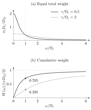
Equal total weight does not imply equal weight inside a finite window. The two curves have the same $D_D$ and rates $\gamma/\Omega_c=0.5$ and $2$. The vertical guide marks the cutoff; the lower panel integrates each curve, with the complete positive-frequency weight normalized to one.

One sometimes defines an effective carrier count per volume by $n_{\mathrm{eff}}(\Omega_c)=2m_{\mathrm{ref}}W(\Omega_c)/(\pi e^2)$. This is a way to quote an area using a declared reference mass. It is not necessarily a particle density. Carrier number, band curvature, mass renormalization, scattering width and transfers between intraband and interband sectors can all affect an inferred low-energy weight.

What spectral-weight transfer can establish

Compare spectra in the same polarization, geometry and normalization, then examine the difference of cumulative integrals over a range of cutoffs. A recovery plateau can identify an energy scale over which the observed redistribution closes, subject to extrapolation errors. A single chosen cutoff cannot establish that closure. A restricted lattice sum may also change because its contact expectation changes, while the full continuum sum remains compatible with fixed total electron density.

Broad redistribution and suppressed coherent weight are useful evidence for correlations when compared with a specified band reference and other probes; they do not uniquely determine a self-energy or interaction mechanism. Basov et al. (2011) survey this use of optical data. A fit to frequency-dependent scattering and mass functions likewise requires an assigned intraband sector and weight. Unremoved interband absorption can produce apparent frequency dependence even without the proposed many-body mechanism.

Condensate weight and the missing-area relation

In a superconducting state, a dissipationless response can produce $\pi D_{\delta,S}\delta(\omega)$ in $\sigma_1$ and $D_{\delta,S}/\omega$ in $\sigma_2$. A clean normal conductor can also carry an optical delta; the pole alone does not prove superconductivity. Identifying it with the London superfluid stiffness requires the appropriate phase, response limit and absence of an additional ballistic contribution.

Subtract the complete optical sum of a normal reference $N$ from that of a superconducting state $S$. Allow both to have a delta and allow their lattice contact terms to differ. The two sum rules then give

$$D_{\delta,S}-D_{\delta,N} ={}\frac2\pi\int_0^\infty d\omega\, \left[\sigma_{1,N}^{\mathrm{reg}}-\sigma_{1,S}^{\mathrm{reg}}\right] +D^{\mathrm{dia}}_S-D^{\mathrm{dia}}_N.$$

When the normal reference has no delta and the contact terms are equal, the lost finite-frequency area determines $D_{\delta,S}$. This is the usual missing-area form of the Ferrell–Glover–Tinkham sum rule (Ferrell and Glover, 1958; Tinkham and Ferrell, 1959). A finite cutoff replaces the integral only after the missing area has converged, or after the omitted difference is bounded. The temperature and magnetic-field extrapolation used to construct a normal reference is part of that claim.

In the isotropic local London regime, when this pole is the superfluid contribution,

$$D_s=\frac1{\mu_0\lambda_L^2}, \qquad \sigma_{2,s}(\omega)=\frac{D_s}{\omega}.$$

London Theory explains magnetic screening and penetration depth. Nonlocality, vortices, normal-fluid absorption and anisotropy require additional response information. An optical onset near a pair-breaking scale also depends on selection rules, disorder and gap structure; BCS Theory provides the microscopic benchmark. Neither a missing absorption band nor a $1/\omega$ reactive tail is a complete phase diagnosis on its own.

Conductivity, dielectric response and the optical experiment

If $\sigma$ contains all material polarization currents in a local bulk model, its relative dielectric function is

$$\epsilon_r(\omega)=1+\frac{i\sigma(\omega)}{\epsilon_0\omega}.$$

If some high-energy polarization has instead been assigned to a background $\epsilon_b(\omega)$, use $\epsilon_r=\epsilon_b+i\sigma_{\mathrm{retained}}/(\epsilon_0\omega)$. Do not count the same interband contribution in both terms. For a real background in the window, $\epsilon_2=\sigma_1/(\epsilon_0\omega)$ and $\epsilon_1=\epsilon_b-\sigma_2/(\epsilon_0\omega)$.

Dielectric Response, Screening, and Loss distinguishes local optical response from longitudinal screening and the inverse-response loss function. Maxwell boundary conditions then connect the material response to reflectance, transmission and surface impedance. Film thickness, substrate response, polarization and interference belong to that forward problem. For a sheet, the sheet conductance enters boundary conditions directly; assigning it a fictitious bulk thickness is not required.

Terahertz and Infrared Probes and Raman and Optical Spectroscopy develop the corresponding measurements. Their inferred spectra must obey the same causal and passive-response constraints, with any partial-sum conclusion tested across integration cutoffs.

Exercises

More low-frequency weight without more carriers

Two spectra have the same Drude weight $D_D$ but rates $\gamma_A=\Omega_c/2$ and $\gamma_B=2\Omega_c$. Find their captured weight fractions and dc-conductivity ratio. Can the finite-window area difference be interpreted as a change in $n/m^*$?

Solution

The fractions are

$$\begin{aligned} F_A&=\frac2\pi\arctan2\simeq0.704833,\\ F_B&=\frac2\pi\arctan\frac12\simeq0.295167. \end{aligned}$$

Since $\sigma_{\mathrm{dc}}=D_D/\gamma$, the dc ratio is $\sigma_A/\sigma_B=4$. Yet both complete areas equal $\pi D_D/2$. The area ratio inside this window is about $2.39$ and is caused entirely by narrowing; interpreting it as a change in $n/m^*$ would be wrong for these spectra.

A passive oscillator with negative reactive response

For the Lorentz term in the text, find $\sigma_1$ and $\sigma_2$ at $\omega=\omega_0$ and in the low-frequency limit. Explain why $\sigma_2<0$ below resonance does not violate passivity.

Solution

Multiplying by the complex-conjugate denominator gives

$$\sigma_{2,L}=-\frac{D_L\omega(\omega_0^2-\omega^2)} {(\omega_0^2-\omega^2)^2+\Gamma^2\omega^2}.$$

At resonance, $\sigma_{1,L}=D_L/\Gamma$ and $\sigma_{2,L}=0$. At small positive $\omega$, $\sigma_{1,L}\simeq D_L\Gamma\omega^2/\omega_0^4$ and $\sigma_{2,L}\simeq-D_L\omega/\omega_0^2$. Absorbed power depends on the nonnegative real part. The negative imaginary part represents the phase of a bound polarization current, not energy production.

Positive diagonal entries are not enough

At a fixed positive frequency consider

$$\boldsymbol\sigma= \begin{pmatrix}s&ia\\-ia&s\end{pmatrix}, \qquad s>0,\quad a\in\mathbb R.$$

Find the passivity condition and the absorption for the two unit circular polarizations. Compare with a real antisymmetric Hall contribution.

Solution

This matrix is Hermitian. Its eigenvectors $\mathbf e_\pm=(1,\pm i)^T/\sqrt2$ have eigenvalues $s\mp a$, respectively. For field amplitude $E_0$, the powers are $|E_0|^2(s\mp a)/2$. Passivity for every polarization requires $|a|\le s$; positive diagonal entries alone do not ensure it.

A real antisymmetric matrix $\begin{pmatrix}0&h\\-h&0\end{pmatrix}$ is anti-Hermitian and contributes zero to the absorbed-power quadratic form. This is why an off-diagonal response must be analyzed with its phase and tensor structure, not with a componentwise positivity rule.

A contact correction to missing area

Measure all stiffnesses in one common unit $D_0$. A model has $D_N^{\mathrm{dia}}=5D_0$, $D_S^{\mathrm{dia}}=4D_0$, $D_{\delta,N}=0$ and regular missing area $3\pi D_0/2$. Find the superconducting delta weight and check both full sums.

Solution

The identity gives

$$D_{\delta,S}=3D_0+(4-5)D_0=2D_0.$$

The normal regular area is $5\pi D_0/2$. The superconducting regular area is smaller by $3\pi D_0/2$, hence equals $\pi D_0$. Adding half the delta weight, $\pi D_{\delta,S}/2=\pi D_0$, yields a superconducting full area $2\pi D_0=\pi D_S^{\mathrm{dia}}/2$. Ignoring the contact change would incorrectly assign $3D_0$ to the pole.

References

• Basov, Dimitri N., Richard D. Averitt, Dirk van der Marel, Martin Dressel, and Kristjan Haule. “Electrodynamics of Correlated Electron Materials.” Reviews of Modern Physics 83, 471–541 (2011). doi:10.1103/RevModPhys.83.471; arXiv:1106.2309. Optical weight, correlation-sensitive redistribution and the limits of effective scattering and mass descriptions.
• Ferrell, Richard A., and Rolfe E. Glover III. “Conductivity of Superconducting Films: A Sum Rule.” Physical Review 109, 1398–1399 (1958). doi:10.1103/PhysRev.109.1398. The missing-area connection between regular absorption and supercurrent response.
• Tinkham, Michael, and Richard A. Ferrell. “Determination of the Superconducting Skin Depth from the Energy Gap and Sum Rule.” Physical Review Letters 2, 331–333 (1959). doi:10.1103/PhysRevLett.2.331. Causal optical response, sum rules and superconducting penetration depth, including spatially nonlocal response.