Landauer–Büttiker Formalism

The Landauer–Büttiker formalism computes currents between reservoirs from the scattering of their occupied incoming channels. For a stationary, elastic, normal conductor, the central object is a unitary scattering matrix. Reservoirs set occupations; the device mixes amplitudes; measured currents follow after summing outgoing fluxes. This description naturally gives a terminal conductance, rather than a local conductivity assigned to the coherent region.

Here the scatterer is noninteracting, or described by a justified effective one-particle Hamiltonian; an arbitrary strongly interacting device does not acquire a Landauer description merely by fitting a transmission curve. Conductance Quantization connects channels to observed plateaus. Mesoscopic Transport develops sequential charge-state kinetics and counting statistics when that description is more appropriate.

Required background. S-Matrix supplies channel scattering and unitarity; Fermi–Dirac Statistics supplies reservoir occupations; Chemical Potential supplies the particle-exchange and energy-reference conventions.

Helpful background. What Is Mesoscopic Physics? supplies the relevant length scales; Conductance Quantization supplies mode counting; Quantum Coherence in Conductors supplies interference and averaging; Mesoscopic Transport supplies the kinetic alternative.

Reservoirs, channels and terminal polarity

Lead $\alpha$ joins an ideal reservoir to the scattering region. Far from the region it supports $N_\alpha(E)$ incoming and the same number of outgoing propagating channels. Count every resolved spin, valley or other internal state once. Evanescent modes can affect the scattering solution but are not independent asymptotic flux channels. A chiral edge network must include its contacts and return paths so that all incoming and outgoing fluxes are included.

The reservoir injects mutually incoherent channels with occupation

$$f_\alpha(E)=\frac{1}{1+\exp[(E-\mu_\alpha)/(k_BT_\alpha)]}.$$

Here $E$ is a common total one-particle energy and $\mu_\alpha$ is the electrochemical reservoir potential in that energy reference. Electric potential energy must not be added to it a second time. Outgoing particles are absorbed and equilibrate in the reservoir; their phases are not returned to the device.

Use signed carrier charge $q=-e$ for electrons. Define $J_{N\alpha}$ as particle current out of reservoir $\alpha$ into the device, and define conventional charge current in that same geometrical direction by $I_\alpha=qJ_{N\alpha}$. Relative to equilibrium $\mu$, set

$$V_\alpha=\frac{\mu_\alpha-\mu}{q}.$$

This is the physical electrochemical voltage used in Thermoelectric Response. Increasing an electron reservoir’s $\mu_\alpha$ makes this $V_\alpha$ more negative. The positive-bias convention $V=(\mu_S-\mu_D)/e$ used in the plateau article instead equals $-(V_S-V_D)$, and that article’s drain-to-source current is $-I_S$. Both choices give positive conductance when the voltage and current signs are translated together.

From unitary scattering to current

At each energy, write $b=Sa$, with $a$ incoming and $b$ outgoing channel amplitudes normalized to unit particle flux. The block $S_{\alpha\beta}$ maps incoming lead $\beta$ to outgoing lead $\alpha$. Define the dimensionless total transmission, including reflection when the indices coincide,

$$\begin{aligned} \mathcal T_{\alpha\beta} &=\operatorname{Tr}(S_{\alpha\beta}^\dagger S_{\alpha\beta}),\\ A_{\alpha\beta} &=N_\alpha\delta_{\alpha\beta}-\mathcal T_{\alpha\beta}. \end{aligned}$$

The trace sums probabilities over all incoming and outgoing channels in the two leads. It can exceed one; an individual transmission eigenvalue cannot. If scattering amplitudes were normalized to wave amplitude instead, velocity ratios must first convert them into flux amplitudes.

Unitarity on the complete propagating-channel space gives two different sum rules:

$$\begin{aligned} \sum_\alpha\mathcal T_{\alpha\beta}&=N_\beta, &\sum_\beta\mathcal T_{\alpha\beta}&=N_\alpha,\\ \sum_\alpha A_{\alpha\beta}&=0, &\sum_\beta A_{\alpha\beta}&=0. \end{aligned}$$

The first counts where a given incoming channel exits; the second counts the incoming contributions to an outgoing lead. Checking only columns misses the condition that prevents a current at common occupation.

For example, a single incoming electron may have amplitudes to leave through several contacts. Probabilities from that one channel sum to one, even though its paths interfere inside the device. Different occupied incoming channels are then summed incoherently because the reservoirs do not fix their relative phases. Thus coherent scattering within the device and incoherent injection from reservoirs are compatible.

One occupied incoming channel contributes particle flux $dE/h$; its velocity cancels its one-dimensional density of states, as derived in Conductance Quantization. The outgoing flux into lead $\alpha$ is therefore $h^{-1}\sum_\beta\mathcal T_{\alpha\beta}f_\beta\,dE$. Subtracting it from injection gives

$$\begin{aligned} J_{N\alpha}&=\frac1h\int dE\sum_\beta A_{\alpha\beta}(E)f_\beta(E),\\ I_\alpha&=qJ_{N\alpha}. \end{aligned}$$

Integrate over all propagating energies, with channel counts and transmissions zero where channels are closed. Column sums ensure $\sum_\alpha I_\alpha=0$; row sums ensure every terminal current vanishes when all $f_\alpha$ coincide. Reflection is essential to both checks. This terminal construction underlies Büttiker’s multi-probe formulation and its reciprocity relations [Büttiker, 1986a].

Two terminals and transmission eigenvalues

For two normal leads, unitarity gives equal total left-to-right and right-to-left transmission even at fixed magnetic field. Set $t=S_{21}$ and $\mathcal T=\operatorname{Tr}t^\dagger t=\sum_n\tau_n$, where $0\leq\tau_n\leq1$. Unequal lead channel counts only add zero eigenvalues to the larger channel space. Then

$$\begin{aligned} I_1&=\frac qh\int dE\,\mathcal T(E)[f_1(E)-f_2(E)],\\ I_2&=-I_1. \end{aligned}$$

The eigenchannels diagonalize transmission probability; they need not coincide with the uncoupled transverse modes in a chosen lead basis. Their utility and bounds follow from the unitary scattering construction [Beenakker, 1997].

At common temperature $T$ and small $\Delta V=V_1-V_2$, expand $f_1-f_2=q\Delta V(-\partial_Ef)$:

$$G=\frac{q^2}{h}\int dE\, \mathcal T(E)(-\partial_Ef).$$

At zero temperature this samples $E=\mu$. At finite temperature it averages over an energy window of width of order $k_BT$; replacing it by $\mathcal T(\mu)$ needs a slowly varying transmission. No extra factor of two is added if spin was already counted in $n$. An orbital-channel convention may extract a degeneracy factor only when those copies really share the same transmission.

Conductance matrices and reciprocity

In isothermal linear response, define $\overline A=\int dE\,(-\partial_Ef)A(E)$ at equilibrium. The terminal conductance matrix is

$$I_\alpha=\sum_\beta G_{\alpha\beta}V_\beta, \qquad G_{\alpha\beta}=\frac{q^2}{h}\overline A_{\alpha\beta}.$$

Its column sums vanish by charge conservation and its row sums vanish by invariance under a common voltage shift. Thus the full matrix is singular: choose a reference potential, then solve on the remaining connected terminals. A disconnected component requires its own reference or further physical boundary data.

The same sum rules prove isothermal passivity. With $\overline{\mathcal T}_{\alpha\beta}=\int dE\,(-\partial_Ef)\mathcal T_{\alpha\beta}(E)$,

$$\sum_\alpha V_\alpha I_\alpha =\frac{q^2}{2h}\sum_{\alpha\beta} \overline{\mathcal T}_{\alpha\beta}(V_\alpha-V_\beta)^2 \geq0.$$

This uses balanced row and column sums, not symmetry of $\mathcal T$ at a fixed field. It bounds total electrical dissipation without requiring each transfer resistance to be positive.

The row identity guarantees gauge invariance of the linear response around a common equilibrium. For finite changes, a true common electrostatic shift also shifts the device potential, lead thresholds and energy reference. Shifting only the reservoir chemical potentials while holding the scatterer fixed can change its occupation relative to a gate; that is a different physical experiment. A bias-dependent Hartree potential requires a self-consistent scattering problem.

If microscopic dynamics is reversible, tracing over the time-reversed channel partners gives

$$\begin{aligned} \mathcal T_{\alpha\beta}(B,\mathbf M) &=\mathcal T_{\beta\alpha}(-B,-\mathbf M),\\ G_{\alpha\beta}(B,\mathbf M) &=G_{\beta\alpha}(-B,-\mathbf M). \end{aligned}$$

All time-reversal-odd controls, including magnetization $\mathbf M$, must reverse. Consequently a two-terminal linear conductance is even under that full reversal. A four-terminal resistance need not be even at fixed contact roles. With $I_\alpha=I$, $I_\beta=-I$ and all other terminal currents zero, define $R_{\alpha\beta,\gamma\delta}=(V_\gamma-V_\delta)/I$. Reciprocity reads

$$R_{\alpha\beta,\gamma\delta}(B,\mathbf M) =R_{\gamma\delta,\alpha\beta}(-B,-\mathbf M).$$

These lead-exchange relations are central to Büttiker’s four-terminal analysis [Büttiker, 1986a]. They assume corresponding equilibrium states and a linear measurement, not arbitrary hysteretic sweeps or nonlinear differential resistances.

Contacts, floating probes and loss of coherence

A perfect coherent connection with $N$ resolved channels has two-terminal resistance $h/(q^2N)$. Finite resistance does not require dissipative scattering inside that connection: the current is set by reservoir injection, and nonequilibrium outgoing distributions relax in the reservoirs. Conductance Quantization discusses the plateau and contact interpretation in detail.

A voltage probe is an additional reservoir, not an instruction to sample a pre-existing local voltage without disturbance. For fixed probe temperature impose $I_p=0$ and solve for its voltage. Its carriers are still absorbed and re-emitted; zero net charge current does not mean zero exchange or zero heat flow. Büttiker’s reservoir construction supplies a controlled model of such incoherent reinjection [Büttiker, 1986b].

For several isothermal probes $P$ and measured terminals $A$, partition the full matrix. If $G_{PP}$ is invertible after fixing the relevant reference,

$$\begin{aligned} V_P&=-G_{PP}^{-1}G_{PA}V_A,\\ G_{\mathrm{eff}} &=G_{AA}-G_{AP}G_{PP}^{-1}G_{PA}. \end{aligned}$$

The Schur complement preserves conservation, gauge invariance and reciprocity when the original matrix and boundary conditions have them. It describes the sample with those probes attached. A four-terminal resistance depends on their coupling and channel selectivity; it is not obtained by subtracting a universal contact resistance from every coherent network. Negative nonlocal transfer resistance is compatible with positive total dissipation.

Different fictitious probes impose different constraints [Förster et al., 2007]:

Probe	Condition	What can relax
Isothermal voltage probe	Integrated $I_p=0$; fixed $T_p$	Energy and phase
Floating thermal probe	$I_p=J_{Qp}=0$; solve $V_p,T_p$	Distribution equilibrates internally
Elastic dephasing probe	Zero particle flux at each $E$	Phase, without energy exchange

For a single dephasing probe the last condition gives

$$f_p(E)= \frac{\sum_{\beta\ne p}\mathcal T_{p\beta}(E)f_\beta(E)} {N_p(E)-\mathcal T_{pp}(E)}.$$

This is usually a non-Fermi distribution; the denominator must be nonzero where the probe is connected. Several probes require an energy-by-energy linear system. Do not equate all probe constructions with phase averaging, or infer their noise by imposing only the average-current constraints.

Heat currents and thermoelectric transport

The energy flux out of reservoir $\alpha$ uses the same $E$ as its occupation. Heat excludes the chemical work carried with particles:

$$\begin{aligned} J_{E\alpha}&=\frac1h\int dE\,E\sum_\beta A_{\alpha\beta}f_\beta,\\ J_{Q\alpha}&=J_{E\alpha}-\mu_\alpha J_{N\alpha}. \end{aligned}$$

Stationary elastic scattering conserves total energy, $\sum_\alpha J_{E\alpha}=0$. It does not conserve the sum of reservoir heat currents:

$$\sum_\alpha J_{Q\alpha} =-\sum_\alpha V_\alpha I_\alpha.$$

With our outward-current convention, positive electrical power is deposited as negative total outward heat. Each reservoir has its own chemical subtraction; replacing every $\mu_\alpha$ by equilibrium $\mu$ would miss Joule heating. A particular reservoir can cool even while the total dissipated power is positive.

Linearizing around $\mu,T$ introduces energy-moment matrices

$$L^{(n)}_{\alpha\beta} =\frac1h\int dE\,(E-\mu)^n A_{\alpha\beta}(E)(-\partial_Ef).$$

They give

$$\begin{aligned} I_\alpha&=\sum_\beta\left[ q^2L^{(0)}_{\alpha\beta}V_\beta +\frac qT L^{(1)}_{\alpha\beta}\delta T_\beta\right],\\ J_{Q\alpha}&=\sum_\beta\left[ qL^{(1)}_{\alpha\beta}V_\beta +\frac1T L^{(2)}_{\alpha\beta}\delta T_\beta\right]. \end{aligned}$$

Butcher [1990] develops this multi-terminal heat extension and its reciprocal structure. The electrical Joule term is second order in voltage and is therefore absent from this linear heat equation. A floating thermal probe must be eliminated from the full charge/heat system, not merely from $G$.

For two terminals replace $A$ by the scalar total transmission in the moment integral and call the moments $\ell_n$. With $I=I_1$, $\Delta T=T_1-T_2$ and $\Delta V=V_1-V_2$,

$$\begin{aligned} G&=q^2\ell_0,\\ S&\equiv-\left.\frac{\Delta V}{\Delta T}\right|_{I=0} =\frac{\ell_1}{qT\ell_0},\\ K_{I=0}&=\frac1T\left(\ell_2-\frac{\ell_1^2}{\ell_0}\right). \end{aligned}$$

Here $K$ is thermal conductance in W/K, not bulk thermal conductivity. The nonnegative weight $\mathcal T(-f')/h$ makes $\ell_0\ell_2-\ell_1^2\geq0$ by Cauchy–Schwarz, so the electronic open-circuit $K$ is nonnegative when $\ell_0>0$. Phonons and other independent heat paths must be added separately. These are the coherent-terminal counterparts of the bulk coefficients in Thermoelectric Response.

Choosing the complete transport problem

An edge-state network is one application of this terminal description; Integer Quantum Hall Effect explains its topology and chirality. Superconducting terminals require electron–hole channels and the charge transferred to the condensate, as developed in Proximity and Andreev Physics. Doubling the charge in the normal-state formula does not supply those processes.

Static elastic disorder and multiple reflections fit within $S$ and can produce localization. Strong charging, genuinely inelastic collisions and interacting nonequilibrium correlations require additional theory. A one-particle effective transmission is valid only with a derivation appropriate to that regime. Time-dependent driving requires sidebands and energy exchange; finite-frequency admittance also needs charge accumulation and displacement currents. Neither follows by attaching an arbitrary frequency argument to the dc conductance matrix.

Exercises

1. A zero-current probe that absorbs heat

Take three single-channel leads with $S_{\alpha\beta}=3^{-1/2}\exp[2\pi i(\alpha-1)(\beta-1)/3]$. Let the transmission be constant throughout the small bias window, $T_\alpha=0$, $V_1=V$, $V_2=0$, and lead 3 be a floating isothermal voltage probe. Find its voltage, the two-terminal conductance and the heat deposited in the probe.

Solution

The discrete Fourier matrix is unitary and $\mathcal T_{\alpha\beta}=1/3$, including reflection. With $g=q^2/h$,

$$I_\alpha=g\left(V_\alpha-\frac{V_1+V_2+V_3}{3}\right).$$

Thus $V_3=V/2$, $I_1=gV/2=-I_2$ and $G_{\mathrm{eff}}=g/2$. For energy-independent scattering at zero temperature, direct integration of the heat formula yields

$$J_{Q\alpha}=-\frac g2\sum_\beta \mathcal T_{\alpha\beta}(V_\alpha-V_\beta)^2.$$

Therefore $J_{Q3}=-gV^2/12$: heat enters the nominally zero-current probe. The other heat currents are each $-5gV^2/24$. Their sum is $-gV^2/2=-VI_1$, as required. A probe floating in both voltage and temperature would obey a different boundary problem.

2. Coherent barriers versus a new reservoir

Two single-channel barriers have transmission probabilities $\tau_1,\tau_2$ and reflection probabilities $r_j=1-\tau_j$. Let $\theta$ include the propagation and reflection phase of a round trip. Sum the repeated-reflection amplitudes and compare, for $\tau_1=\tau_2=1/2$, a coherent device, uniform phase averaging and two barriers joined by a fully absorbing equilibrating reservoir. Use infinitesimal isothermal bias and broad, constant barrier transmissions.

Solution

The amplitude series has ratio $\sqrt{r_1r_2}e^{i\theta}$; hence

$$\tau_{\mathrm{coh}}(\theta)= \frac{\tau_1\tau_2}{1+r_1r_2-2\sqrt{r_1r_2}\cos\theta}.$$

Equal half-transparent barriers give $\tau_{\mathrm{coh}}(0)=1$ and $\tau_{\mathrm{coh}}(\pi)=1/9$. Uniform averaging gives

$$\langle\tau_{\mathrm{coh}}\rangle_\theta =\frac{\tau_1\tau_2}{1-r_1r_2}=\frac13.$$

For the inserted reservoir, the two two-terminal conductances are $g\tau_1$ and $g\tau_2$. The zero-current reservoir voltage gives a series conductance $G=g\tau_1\tau_2/(\tau_1+\tau_2)=g/4$. This is a different contact geometry and an additional equilibration boundary, not the same device with its interference fringes erased. In particular, the reservoir adds resistance even if both barriers become perfectly transmitting.

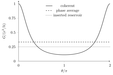
For the two half-transparent barriers, $G/g=1/(5-4\cos\theta)$. The dashed line is its uniform phase average, $1/3$. Replacing the intervening coherent region by a fully absorbing reservoir produces the dotted value $1/4$; it changes the contact problem as well as removing interference.

3. A directed four-terminal network

One resolved channel propagates in the sequence $1\to2\to3\to4\to1$, with complete absorption at every reservoir. Apply $I_1=I$, $I_3=-I$, $I_2=I_4=0$. Find $R_{13,24}$ and compare reversal of propagation at fixed lead roles with reciprocal exchange of current and voltage leads. This is a terminal-network exercise, without assigning its circulation to a particular magnetic-field sign.

Solution

The nonzero probabilities are $\mathcal T_{21}=\mathcal T_{32}=\mathcal T_{43}=\mathcal T_{14}=1$. Then $I_\alpha=g(V_\alpha-V_{\alpha-1})$ cyclically. With $V_3=0$, one finds

$$\begin{aligned} V_1&=V_2=I/g,\qquad V_3=V_4=0,\\ R_{13,24}&=1/g. \end{aligned}$$

Reverse the arrows while keeping the same driven contacts: now $V_2=V_3$ and $V_4=V_1$, giving $R_{13,24}^{\mathrm{rev}}=-1/g$. Instead drive $2\to4$ in the reversed network and measure $V_1-V_3$. The result is $R_{24,13}^{\mathrm{rev}}=1/g$, equal to the original resistance. A four-terminal signal need not be even under reversal to obey reciprocity.

4. A thermal channel and its bias heat

Let a two-terminal normal device have constant total transmission $\mathcal T_0$ throughout a broad window containing $\mu$, several $k_BT$, and the small bias. Find $G$, $S$ and $K_{I=0}$ to exponentially small band-edge corrections. At equal reservoir temperatures, also find the Joule heat entering each contact for a voltage difference $\Delta V$.

Solution

The Fermi-window integrals give

$$\begin{aligned} \ell_0&=\frac{\mathcal T_0}{h},\qquad \ell_1=0,\\ \ell_2&=\frac{\pi^2(k_BT)^2\mathcal T_0}{3h}. \end{aligned}$$

Thus $G=q^2\mathcal T_0/h$, $S=0$ and $K_{I=0}=\pi^2k_B^2T\mathcal T_0/(3h)$. The Lorenz ratio is $K_{I=0}/(GT)=\pi^2k_B^2/(3q^2)$. This is a channel conductance relation under the stated energy-independent transmission assumption.

At equal temperatures the exact energy integral gives

$$J_{Q1}=J_{Q2}=-\frac12G(\Delta V)^2.$$

The two reservoirs share the heat equally in this symmetric energy-independent model. Energy-dependent transmission generally changes that partition and can add Peltier cooling or heating. Zero heat generated in the elastic scattering region does not imply zero heat delivered to the contacts.

References

• Beenakker, C. W. J., “Random-matrix theory of quantum transport,” Reviews of Modern Physics 69, 731–808 (1997), doi:10.1103/RevModPhys.69.731; author preprint — flux-unitary scattering, transmission eigenvalues and the normal-state Landauer conductance.
• Butcher, P. N., “Thermal and electrical transport formalism for electronic microstructures with many terminals,” Journal of Physics: Condensed Matter 2, 4869–4878 (1990), doi:10.1088/0953-8984/2/22/008 — reservoir heat currents, thermoelectric moments and multi-terminal reciprocity.
• Büttiker, M., “Four-Terminal Phase-Coherent Conductance,” Physical Review Letters 57, 1761–1764 (1986a), doi:10.1103/PhysRevLett.57.1761 — terminal-current matrices and exchange of current and voltage leads under reversal.
• Büttiker, M., “Role of quantum coherence in series resistors,” Physical Review B 33, 3020–3026 (1986b), doi:10.1103/PhysRevB.33.3020 — reservoir models of incoherent scattering and the importance of the contact construction.
• Förster, H., Samuelsson, P., Pilgram, S., and Büttiker, M., “Voltage and dephasing probes in mesoscopic conductors: A study of full-counting statistics,” Physical Review B 75, 035340 (2007), doi:10.1103/PhysRevB.75.035340; author preprint — distinct probe constraints and the limits of identifying probes with phase averaging.