Drude Theory

Drude theory is the single-relaxation-time model of charge-current response. It assumes that a carrier’s mean drift momentum accelerates under an electric field and relaxes exponentially toward equilibrium:

$$\frac{d\mathbf p_d}{dt} = q\mathbf E - \frac{\mathbf p_d}{\tau}.$$

For an isotropic parabolic band, $\mathbf p_d=m^*\mathbf v_d$. The resulting dc conductivity is

$$\sigma_0 = \frac{nq^2\tau}{m^*}.$$

This formula looks classical, but its successful modern use is usually Drude–Sommerfeld: carrier density comes from Fermi statistics and band filling, the response-appropriate $m^*$ from band structure and any necessary interaction corrections, and $\tau$ from momentum-relaxing scattering near the Fermi surface. The model does not predict those inputs. It organizes them into a low-frequency response.

The derivation below connects the drift equation to dc, ac and Hall response, then tests what can be inferred from a fitted relaxation time. Transport coefficients explains the broader transport limits, Kubo formula gives the correlation-function formulation, and Effective mass distinguishes the masses measured by different probes.

Required background. Effective Mass supplies the response-specific mass distinctions used here without rederivation.

Helpful background. Fermi Surface supplies low-energy phase space, Metals, Insulators, and Semiconductors supplies carrier and filling classification, and Transport Coefficients Preview supplies the bulk, ballistic, hydrodynamic, and limit-order taxonomy.

Drude momentum relaxation and current

Let $q$ be the signed carrier charge. Thus $q=-e$ for an electron and $q=+e$ for a hole. The microscopic carrier velocity can be large even in equilibrium, but opposite directions cancel. $\mathbf v_d$ denotes only the small nonequilibrium drift average.

For an isotropic band and zero magnetic field,

$$m^* \frac{d\mathbf v_d}{dt} = q\mathbf E(t) - \frac{m^*\mathbf v_d}{\tau}.$$

The relaxation term asserts:

• linear response in the drift velocity;
• local, memoryless damping;
• one momentum-relaxation time $\tau$;
• a fixed carrier density and effective mass;
• spatially uniform response;
• no distinction among directions, bands, or points on the Fermi surface.

Those are model assumptions, not definitions of a metal.

Time-domain solution

After transients from the remote past have decayed,

$$\mathbf v_d(t) = \frac{q}{m^*} \int_{-\infty}^{t} dt'\, e^{-(t-t')/\tau} \mathbf E(t').$$

The response kernel is causal: only earlier fields contribute.

If a constant field $\mathbf E_0$ is switched on at $t=0$ and the initial drift is zero,

$$\mathbf v_d(t) = \frac{q\tau}{m^*} \mathbf E_0 \left( 1-e^{-t/\tau} \right).$$

If the field is switched off after steady state is reached, the current decays as $e^{-t/\tau}$. This is the operational meaning of the model’s relaxation time.

What relaxes

$\tau$ is a transport momentum-relaxation time. It need not equal:

• the interval between all microscopic collisions;
• a single-particle quantum lifetime from spectral broadening;
• a phase-coherence time;
• an energy-relaxation time;
• a recombination time;
• an escape time from a finite device.

A collision that changes momentum only slightly can strongly broaden a single-particle phase while relaxing current inefficiently. Naming the lifetime is part of reporting it.

DC Conductivity

In a time-independent field, the steady drift is

$$\mathbf v_d = \frac{q\tau}{m^*} \mathbf E.$$

The current density is

$$\mathbf j = nq\mathbf v_d.$$

Although electron drift is opposite to $\mathbf E$, multiplying by the negative electron charge makes the conventional current parallel to $\mathbf E$. Therefore

$$\mathbf j = \sigma_0\mathbf E, \qquad \sigma_0 = \frac{nq^2\tau}{m^*}.$$

The resistivity is

$$\rho_0 = \frac{1}{\sigma_0} = \frac{m^*}{nq^2\tau}.$$

Define the positive mobility

$$\mu = \frac{|q|\tau}{m^*}.$$

Then

$$\sigma_0 = n|q|\mu.$$

Conductivity is a bulk coefficient. Conductance also depends on sample geometry and contacts. For a uniform bar of length $L$ and cross-sectional area $A$,

$$G = \sigma_0 \frac{A}{L},$$

only when current distribution and contact effects permit the elementary geometry reduction.

Classical Equation, Quantum Inputs

The original Drude model treated carriers as a classical gas. That picture gives incorrect electronic heat capacity and misses Pauli blocking, band structure, and Fermi-surface geometry. Modern use keeps the momentum-balance equation while replacing its inputs.

Carrier density

$n$ is obtained from the occupied electronic states, not from a classical Maxwell distribution. In a simple monovalent metal it may be comparable to one carrier per atom; in a doped semiconductor or semimetal it can be many orders of magnitude smaller. In a multiband system there is no single $n$ unless a reduction is justified.

Effective mass

The mass in a Drude fit is fixed by the current response. For a noninteracting parabolic band it is the band mass; in an interacting crystal it need not equal the quasiparticle mass inferred from a spectral dispersion or heat capacity. Current-vertex corrections matter. Conversely, for a translation-invariant continuum with kinetic energy $p^2/(2m_0)$ and interactions depending only on relative coordinates, the uniform current is $q\mathbf P/m_0$. Its clean weight retains $m_0$, even if quasiparticles have a different effective mass. Kohn’s cyclotron-resonance result illustrates this conservation constraint. A real lattice removes that Galilean-invariance argument.

Fermi velocity and mean free path

In a degenerate metal, the characteristic velocity for transport is the Fermi velocity rather than a classical thermal velocity. The transport mean free path is

$$\ell_{\mathrm{tr}} = v_{\mathrm F}\tau_{\mathrm{tr}}.$$

This connects a time-domain Drude parameter with a spatial semiclassical criterion.

Boltzmann reduction

Boltzmann Transport derives the distribution and collision equation. Its simplest weak-field relaxation-time reduction gives

$$\sigma_{ij} = q^2 \sum_n \int \frac{d^dk}{(2\pi)^d} \left( - \frac{\partial f} {\partial\varepsilon} \right) \times v_{n,i}(\mathbf k) v_{n,j}(\mathbf k) \tau_n(\mathbf k).$$

Only states in the thermal window around the chemical potential contribute through $-\partial f/\partial\varepsilon$. For one isotropic parabolic band and constant $\tau$, the integral reduces to $nq^2\tau/m^*$.

For an isotropic degenerate band, the same physics can be written as an Einstein relation,

$$\sigma = q^2 \rho(E_{\mathrm F}) D,$$

with

$$D = \frac{v_{\mathrm F}^2\tau}{d}.$$

Here $\rho(E_{\mathrm F})$ is the density of states per $d$-dimensional volume, including the degeneracies used in $n$; the displayed reduction uses independent quasiparticles with the same transport time. The Drude and diffusion forms agree only when their masses, state counts, and scattering approximations describe the same carriers.

Tensor Drude Response

For a parabolic band with mass tensor $\mathsf M$ and scalar relaxation time,

$$\frac{d\mathbf v_d}{dt} + \frac{\mathbf v_d}{\tau} = q\mathsf M^{-1}\mathbf E.$$

The dc conductivity tensor is

$$\boldsymbol\sigma_0 = nq^2\tau \mathsf M^{-1}.$$

In principal axes,

$$\sigma_{ii} = \frac{nq^2\tau}{m_i}.$$

If $\tau$ is also anisotropic or momentum dependent, it cannot in general be represented by multiplying $\mathsf M^{-1}$ by one scalar. A measured conductivity anisotropy can come from mass, Fermi-surface geometry, direction-dependent scattering or unequal populations of differently oriented valleys. Changing one scalar density alone does not make an isotropic band anisotropic.

Effective Mass distinguishes the tensor, conductivity, density-of-states, cyclotron, and optical masses used in such reductions.

AC Conductivity

Use the convention

$$\mathbf E(t) = \operatorname{Re} \left[ \mathbf E_\omega e^{-i\omega t} \right].$$

The drift equation gives

$$\mathbf v_\omega = \frac{q/m^*} {\tau^{-1}-i\omega} \mathbf E_\omega.$$

Therefore

$$\sigma(\omega) = \frac{nq^2/m^*} {\tau^{-1}-i\omega} = \frac{\sigma_0} {1-i\omega\tau}.$$

The pole lies at $\omega=-i/\tau$, in the lower half-plane as required for a retarded response.

The dissipative and reactive parts are

$$\operatorname{Re}\sigma(\omega) = \frac{\sigma_0} {1+\omega^2\tau^2},$$ $$\operatorname{Im}\sigma(\omega) = \frac{\sigma_0\omega\tau} {1+\omega^2\tau^2}.$$

The cycle-averaged absorbed power density is

$$\overline P = \frac{1}{2} \operatorname{Re}\sigma(\omega) |\mathbf E_\omega|^2.$$

$\operatorname{Re}\sigma$ is a Lorentzian centered at zero frequency with half width

$$\gamma = \frac{1}{\tau}.$$

For $\omega\tau\ll1$, the current nearly follows the field. For $\omega\tau\gg1$, collisions are too slow to establish the dc drift during one cycle and the response is mainly reactive:

$$\sigma(\omega) \approx i \frac{nq^2} {m^*\omega}.$$

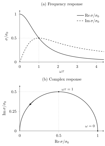
For $\sigma/\sigma_0=(1-i\omega\tau)^{-1}$, the dissipative peak has half width $1/\tau$, while the reactive part peaks at $\omega\tau=1$. At positive frequency the complex conductivity traces the upper semicircle from $\sigma/\sigma_0=1$ toward the origin: $(\operatorname{Re}\sigma/\sigma_0-1/2)^2+(\operatorname{Im}\sigma/\sigma_0)^2=1/4$.

Spectral Weight and the Clean Limit

Write

$$\mathcal D_0 = \frac{nq^2}{m^*}.$$

Then

$$\operatorname{Re}\sigma(\omega) = \mathcal D_0 \frac{\gamma} {\gamma^2+\omega^2}.$$

The positive-frequency intraband area is

$$\int_0^\infty d\omega\, \operatorname{Re}\sigma(\omega) = \frac{\pi}{2} \frac{nq^2}{m^*}.$$

Changing $\tau$ changes the width and height but not this Drude area. In the clean limit,

$$\lim_{\gamma\to0^+} \frac{\gamma} {\gamma^2+\omega^2} = \pi\delta(\omega)$$

on the full frequency axis. Thus

$$\operatorname{Re}\sigma(\omega) \longrightarrow \pi\mathcal D_0 \delta(\omega).$$

Different communities absorb factors of $\pi$ into the definition of “Drude weight.” A quoted Drude weight must include its conductivity convention.

The optical sum of a continuum Hamiltonian uses the mass appearing in that Hamiltonian. For the full nonrelativistic electron problem this is the bare mass $m_0$; for a projected parabolic band it can be $m^*$. A projected model has omitted interband transitions and cannot supply the full-electron sum by extending its Drude curve to arbitrarily high energies. In a lattice, intraband weight can depend on band curvature and interactions.

Sum Rules derives exact integrated spectral constraints. The delta-function distinction between an ideal conductor and an insulator is broader than a finite-$\tau$ fit and connects to Metals, Insulators, and Semiconductors.

Dielectric Function and Plasma Scale

For the $e^{-i\omega t}$ convention,

$$\epsilon(\omega) = \epsilon_\infty + \frac{i\sigma(\omega)} {\epsilon_0\omega}.$$

Define the Drude plasma frequency

$$\omega_p^2 = \frac{nq^2} {\epsilon_0m^*}.$$

Then

$$\epsilon(\omega) = \epsilon_\infty - \frac{\omega_p^2} {\omega \left( \omega+i/\tau \right)}.$$

The zero of the longitudinal dielectric function controls a bulk plasma mode after background screening and damping are included. Reflectivity edges, loss-function peaks, and zeros of $\operatorname{Re}\epsilon$ need not coincide when absorption or interband structure is appreciable.

Plasmons Preview derives the self-consistent modes; Plasmons in Materials explains their dielectric environment and geometry.

Magnetic Field and the Hall Effect

Include a static magnetic field:

$$m^* \frac{d\mathbf v_d}{dt} = q \left( \mathbf E + \mathbf v_d\times\mathbf B \right) - \frac{m^*\mathbf v_d}{\tau}.$$

Take $\mathbf B=B\hat{\mathbf z}$ and define the signed cyclotron frequency and field parameter

$$\omega_c = \frac{qB}{m^*}, \qquad \beta_c = \omega_c\tau.$$

In steady state,

$$\boldsymbol\sigma = \frac{\sigma_0} {1+\beta_c^2} \begin{pmatrix} 1 & \beta_c \\ -\beta_c & 1 \end{pmatrix}.$$

The resistivity tensor is

$$\boldsymbol\rho = \frac{1}{\sigma_0} \begin{pmatrix} 1 & -\beta_c \\ \beta_c & 1 \end{pmatrix}.$$

With the convention

$$R_H = \frac{E_y} {j_xB} = \frac{\rho_{yx}}{B},$$

the single-carrier Hall coefficient is

$$R_H = \frac{1}{nq}.$$

It is negative for electrons and positive for holes. The Hall angle has magnitude

$$|\tan\theta_H| = |\omega_c\tau|.$$

The same one-band isotropic model predicts

$$\rho_{xx}(B) = \rho_0.$$

That is, it has zero transverse magnetoresistance despite a field-dependent $\sigma_{xx}$. Inverting the conductivity tensor matters. Observed magnetoresistance requires additional structure such as multiple carriers, anisotropy, momentum-dependent scattering, open orbits, inhomogeneity, or quantum effects.

Two-carrier response

For carrier species $a$ with positive mobility $\mu_a$ and sign $s_a=\operatorname{sgn}(q_a)$,

$$\sigma_{xx}(B) = \sum_a \frac{ n_a|q_a|\mu_a }{ 1+\mu_a^2B^2 },$$ $$\sigma_{xy}(B) = \sum_a \frac{ s_a n_a|q_a| \mu_a^2B }{ 1+\mu_a^2B^2 }.$$

For electrons of density $n$ and holes of density $p$, the weak-field Hall coefficient is

$$R_H = \frac{ p\mu_h^2 - n\mu_e^2 }{ e \left( p\mu_h+n\mu_e \right)^2 }.$$

The Hall sign is mobility weighted. A positive $R_H$ does not prove that every Fermi-surface sheet is hole-like, and $1/(eR_H)$ is not generally the total carrier density. Fermi Surface develops this warning in the context of electron and hole pockets.

What the Relaxation Time Contains

The Drude equation does not calculate $\tau$. Candidate momentum-relaxing mechanisms include:

• impurities and defects;
• phonons;
• electron–electron Umklapp;
• boundaries and interfaces;
• magnetic fluctuations;
• coupling to other collective modes;
• spatial inhomogeneity.

Transport versus quantum lifetime

For elastic scattering on an isotropic Fermi surface, a representative transport rate is

$$\frac{1}{\tau_{\mathrm{tr}}} = \sum_{\mathbf k'} W_{\mathbf k\mathbf k'} \left( 1-\cos\theta \right).$$

$\theta$ is the angle through which the velocity is scattered. The corresponding single-particle or quantum rate lacks the current-relaxation factor:

$$\frac{1}{\tau_q} = \sum_{\mathbf k'} W_{\mathbf k\mathbf k'}.$$

Forward scattering can make $\tau_{\mathrm{tr}}\gg\tau_q$. Comparing mobility and quantum-oscillation damping as though they measured one lifetime can therefore be misleading.

Matthiessen’s rule

Independent weak scattering channels are often approximated by

$$\frac{1}{\tau_{\mathrm{tr}}} \approx \sum_a \frac{1}{\tau_a}.$$

This is Matthiessen’s rule. It can fail when channels interfere, scattering is strongly energy dependent or anisotropic, the band structure changes with temperature, or one process modifies the distribution sampled by another.

A measured temperature dependence of $\rho$ is not predicted by Drude theory until a microscopic or empirical $\tau(T)$ is supplied.

One slow current-carrying mode

One slowly relaxing quantity that overlaps strongly with the uniform current can give a dominant low-frequency pole,

$$\sigma(\omega)\simeq\frac{\mathcal D_0}{\Gamma-i\omega} +\sigma_{\mathrm{reg}}(\omega).$$

The regular background may be negligible in a restricted frequency range. Microscopic physics then sets the weight and rate; a Drude-like peak does not require the literal classical picture of independent particles between collisions. Rapid momentum-conserving collisions can coexist with slow current decay when current overlaps with an almost conserved momentum. When that overlap vanishes, as it can in a compensated electron–hole system, momentum conservation alone does not protect charge current.

Fermi statistics also changes the interpretation: in a degenerate metal the weak-field occupation change is concentrated near the Fermi surface, even when integration by parts expresses the result through the full density $n$. This is consistent with a small electronic heat capacity. A successful low-frequency fit still constrains response parameters, not an independently established microscopic collision mechanism.

Wiedemann–Franz consistency

For a degenerate Fermi gas with sufficiently elastic, weakly energy-dependent scattering,

$$\frac{\kappa_e} {\sigma T} \longrightarrow L_0, \qquad L_0 = \frac{\pi^2}{3} \left( \frac{k_{\mathrm B}}{e} \right)^2.$$

The quantum Sommerfeld calculation supplies the correct Lorenz number. Deviations can arise from inelastic scattering, additional heat carriers, multiband structure, hydrodynamics, or non-Fermi-liquid behavior.

Extended Drude and Memory Diagnostics

A general causal intraband response can be parameterized as

$$\sigma(\omega) = \frac{\epsilon_0\omega_p^2} {M(\omega)-i\omega},$$

where $M(\omega)$ is a memory function. Ordinary Drude theory takes

$$M(\omega) = \frac{1}{\tau}.$$

Given a chosen intraband plasma frequency, optical analyses sometimes define

$$\frac{1} {\tau_{\mathrm{op}}(\omega)} = \epsilon_0\omega_p^2 \operatorname{Re} \left[ \frac{1}{\sigma(\omega)} \right],$$ $$\frac{m_{\mathrm{op}}(\omega)} {m_b} = - \frac{\epsilon_0\omega_p^2} {\omega} \operatorname{Im} \left[ \frac{1}{\sigma(\omega)} \right].$$

For a perfect Drude response these give $1/\tau$ and $1$. For real data they are derived optical functions, not direct measurements of a microscopic collision clock and mass. Their values depend on the chosen plasma frequency and on how interband, phonon, and collective contributions are subtracted.

Interpreting a Drude fit

Dc resistivity fixes $n\tau/m^*=1/(q^2\rho_0)$, while a resolved complex optical spectrum can constrain a Drude area and width separately. Even optics does not independently determine $n$ and $m^*$. The review by Basov and collaborators discusses why low-energy optical weight and current relaxation have to be interpreted together in correlated materials.

Several bands can contribute different widths, and interband or phonon absorption can overlap them. Their sum can produce a frequency-dependent extended-Drude rate even when each individual band has a constant time; Exercise 4 gives an exact example. A causal fit to both real and imaginary response, checked against dc transport and the partial optical sum, is more informative than fitting one peak. Terahertz and infrared probes explains the sample-stack inversion needed first.

In Hall measurements, field reversal helps separate transverse and longitudinal signals when the material state is unchanged apart from the specified reversal. Magnetic hysteresis or an independently ordered magnetization requires additional care. A nonlinear Hall curve rules out the simplest constant-parameter one-carrier model, but a linear curve alone does not establish it. Hall effect treats multiple carriers and anomalous contributions.

The extended-state drift picture itself fails for localized or hopping carriers. The heuristic condition $k_F\ell_{\mathrm{tr}}\lesssim1$ warns against interpreting a fitted time as well-separated quasiparticle collisions; it is not a universal sharp resistivity bound. Viscous flow, ballistic contacts and nonlocal electrodynamics depend on geometry in ways one local time cannot capture. Large fields can heat carriers or change their state, and Landau quantization can invalidate the smooth classical magnetic response. These limits are developed in Boltzmann transport, weak localization and mesoscopic physics.

A zero-frequency delta weight is broader than superconductivity: a clean normal conductor can also have one. Identifying a superconducting state requires the additional phase and magnetic response discussed in Superfluidity and Superconductivity.

Exercises

1. A consistent parabolic-metal estimate

Take

$$n = 5.0\times10^{28}\,\mathrm{m^{-3}}, \qquad \rho_0 = 2.0\times10^{-8}\,\Omega\,\mathrm m,$$

with $m^*=m_0$ in a three-dimensional spin-degenerate parabolic band at low temperature. Derive $k_F$ and $v_F$ from the density, then estimate $\tau$, mobility and mean free path.

Solution

For this band, state counting gives $k_F=(3\pi^2n)^{1/3}\simeq1.140\times10^{10}\,\mathrm{m^{-1}}$. Consequently $v_F=\hbar k_F/m_0\simeq1.32\times10^6\,\mathrm{m/s}$; the Fermi velocity is not a further independent input. From $\rho_0=m_0/(ne^2\tau)$,

$$\tau = \frac{m_0} {ne^2\rho_0} \approx 3.6\times10^{-14}\,\mathrm s.$$

The mobility is

$$\mu = \frac{e\tau}{m_0} \approx 6.3\times10^{-3}\, \mathrm{m^2\,V^{-1}\,s^{-1}},$$

or about $63\,\mathrm{cm^2\,V^{-1}\,s^{-1}}$. The mean free path is

$$\ell = v_{\mathrm F}\tau \approx 4.7\times10^{-8}\,\mathrm m,$$

about $47\,\mathrm{nm}$. These values inherit the assumed one-band mass and density.

2. Mobility-weighted Hall sign

A compensated semimetal has $n=p$, but $\mu_h=2\mu_e$. What is the sign of its weak-field Hall coefficient?

Solution

For $n=p$,

$$R_H = \frac{ n\mu_h^2-n\mu_e^2 }{ en^2 \left( \mu_h+\mu_e \right)^2 }.$$

Since

$$\mu_h^2-\mu_e^2 = 4\mu_e^2-\mu_e^2 > 0,$$

$R_H$ is positive. The material is exactly carrier compensated, yet the more mobile holes control the weak-field Hall sign.

3. Forward scattering

Suppose scattering is concentrated at a small angle $\theta_0\ll1$. Compare its contributions to $1/\tau_q$ and $1/\tau_{\mathrm{tr}}$.

Solution

The quantum rate counts the event with weight approximately one. The transport rate includes

$$1-\cos\theta_0 \approx \frac{\theta_0^2}{2}.$$

Thus the same forward-scattering channel contributes much less to current relaxation:

$$\frac{ \tau_{\mathrm{tr}}^{-1} }{ \tau_q^{-1} } \sim \frac{\theta_0^2}{2}.$$

Consequently $\tau_{\mathrm{tr}}$ can be much longer than $\tau_q$.

4. Frequency-dependent optical rates from constant-time bands

Two independent carrier bands each have the same weight $D$, with relaxation rates $\Gamma$ and $4\Gamma$. Their conductivities add:

$$\sigma(\omega)=\frac{D}{\Gamma-i\omega} +\frac{D}{4\Gamma-i\omega}.$$

Use the total weight $2D$ to define the optical rate and mass ratio above. Find their dependence on $x=\omega/\Gamma$. Does a frequency-dependent optical rate prove that a band’s microscopic scattering rate depends on frequency?

Solution

First combine the two response functions before inverting:

$$\frac{2D}{\sigma(\omega)} =2\Gamma\frac{(1-ix)(4-ix)}{5-2ix}.$$

The real and imaginary parts give

$$\begin{aligned} \frac{\tau_{\mathrm{op}}^{-1}(\omega)}{\Gamma} &=\frac{40+10x^2}{25+4x^2},\\ \frac{m_{\mathrm{op}}(\omega)}{m_b} &=\frac{34+4x^2}{25+4x^2}. \end{aligned}$$

The rate rises from $1.6\Gamma$ to $2.5\Gamma$, and the mass ratio decreases from $1.36$ to 1, although each band’s microscopic rate is constant. The $x=0$ mass value is its continuous limit. Both original responses are causal and have positive absorption. The derived functions reflect their mixture; they do not identify a unique single-band self-energy or an interaction-induced mass enhancement.

References

• N. W. Ashcroft and N. D. Mermin, Solid State Physics, Holt, Rinehart and Winston, 1976.
• D. N. Basov, R. D. Averitt, D. van der Marel, M. Dressel, and K. Haule, “Electrodynamics of Correlated Electron Materials,” Reviews of Modern Physics 83, 471–541 (2011), doi:10.1103/RevModPhys.83.471.
• M. Dressel and G. Grüner, Electrodynamics of Solids, Cambridge University Press, 2002, doi:10.1017/CBO9780511606168.
• P. Drude, “Zur Elektronentheorie der Metalle,” Annalen der Physik 306, 566–613 (1900), doi:10.1002/andp.19003060312.
• W. Kohn, “Cyclotron Resonance and de Haas-van Alphen Oscillations of an Interacting Electron Gas,” Physical Review 123, 1242–1244 (1961), doi:10.1103/PhysRev.123.1242.
• W. Kohn, “Theory of the Insulating State,” Physical Review 133, A171–A181 (1964), doi:10.1103/PhysRev.133.A171.
• R. Kubo, “Statistical-Mechanical Theory of Irreversible Processes. I. General Theory and Simple Applications to Magnetic and Conduction Problems,” Journal of the Physical Society of Japan 12, 570–586 (1957), doi:10.1143/JPSJ.12.570.
• A. Sommerfeld, “Zur Elektronentheorie der Metalle auf Grund der Fermischen Statistik. I,” Zeitschrift für Physik 47, 1–32 (1928), doi:10.1007/BF01391052.
• J. M. Ziman, Electrons and Phonons: The Theory of Transport Phenomena in Solids, Oxford University Press, 1960; Oxford Classic Texts reissue, 2001, doi:10.1093/acprof:oso/9780198507796.001.0001.