Kubo Formula in Materials

A material conductivity is a response of a physical current to an electric field. A current–current correlator is one ingredient; the Hamiltonian’s explicit dependence on the electromagnetic field supplies another. For a consistently gauged model, the optical conductivity takes the form

$$\begin{aligned} \sigma_{ab}(z)&=\frac{i}{z} \left[D^{\mathrm{dia}}_{ab}-\Pi_{ab}(z)\right],\\ z&=\omega+i0^+. \end{aligned}$$

Here $D^{\mathrm{dia}}$ is the equilibrium contact term and $\Pi$ is the paramagnetic current response per volume, with definitions fixed below. Their relative sign controls gauge cancellation, spectral weight and the distinction between a metal and an insulator. This page develops the implementation for periodic materials. The generic weak-source derivation and Lehmann representation remain in Kubo Formula, following Kubo (1957).

Required background. Kubo Formula supplies the causal response kernel and explicit source derivatives; Density and Current Operators supplies charge continuity and the physical current.

Helpful background. Band Theory Overview supplies Bloch eigenvectors and filling; Sum Rules supplies spectral-weight constraints; Spectral Functions distinguishes one-particle linewidths from transport relaxation.

Gauging a material Hamiltonian

Use SI electromagnetic potentials, signed carrier charge $q$ and a bulk sample volume $V$. For electrons $q=-e$, with $e>0$. The optical limit below is spatially uniform, with time dependence $e^{-i\omega t}$ and $\mathbf E=i\omega\mathbf A$ in a gauge with zero scalar potential. Frequency $\omega$ is an angular frequency; $\hbar\omega$ is an energy. A strictly two-dimensional sheet uses area in place of $V$ and yields sheet conductance. Converting it to a three-dimensional conductivity requires an explicitly chosen thickness.

For a continuum electron, minimal coupling replaces $\mathbf p$ by $\mathbf p-q\mathbf A$. For a localized-orbital lattice model, a corresponding long-wavelength approximation is a Peierls phase on each hopping:

$$\begin{aligned} H[\mathbf A]&=\sum_{ij}t_{ij}[\mathbf A]c_i^\dagger c_j+H_{\mathrm{int}},\\ t_{ij}[\mathbf A]&=t_{ij} \exp\!\left(\frac{iq}{\hbar} \int_{\mathbf r_j}^{\mathbf r_i}\mathbf A\cdot d\boldsymbol\ell\right). \end{aligned}$$

The link runs from the annihilated orbital at $j$ to the created orbital at $i$; $t_{ji}=t_{ij}^*$ includes the reverse hopping. With $c_i\mapsto e^{iq\chi(\mathbf r_i)/\hbar}c_i$ and $\mathbf A\mapsto\mathbf A+\nabla\chi$, the phases cancel in each hopping term. A density–density interaction has no additional explicit $\mathbf A$ dependence in this model. Correlated hopping, nonlocal effective interactions and other projections can require additional source vertices.

Peierls substitution is not a universal formula for every truncated electronic-structure basis. It assumes that the retained orbitals and their positions provide an adequate description of the field coupling. Intra-atomic dipole matrix elements, omitted bands and changes of the orbitals in a field may matter for optical response. The model and the electromagnetic coupling must be justified together.

In a fixed orbital Bloch basis with the physical orbital positions included in its Fourier phases, a uniform potential gives

$$h_{\mathbf A}(\mathbf k) =h\!\left(\mathbf k-\frac{q\mathbf A}{\hbar}\right)$$

within that Peierls model. The derivative is with respect to a wavevector component, not a dimensionless crystal coordinate. If a code uses $k_a a$ as its argument, each derivative needs its corresponding length factor. The lattice coupling and kinetic-energy contact term are illustrated explicitly by Maldague (1977).

Physical current and the contact term

Expand the same Hamiltonian to second order in a uniform potential:

$$H[\mathbf A]={}H_0-\sum_a A_aJ_a^{\mathrm p} +\frac V2\sum_{ab}A_a\widehat D^{\mathrm{dia}}_{ab}A_b+O(A^3).$$

$\mathbf J^{\mathrm p}$ is the spatially integrated paramagnetic charge-current density; it has units of charge times velocity. It is not the current through a specified contact. The physical current density is

$$\begin{aligned} \widehat j_a[\mathbf A]&=-\frac1V\frac{\partial H}{\partial A_a} \\ &=\frac{J_a^{\mathrm p}}V-\sum_b\widehat D^{\mathrm{dia}}_{ab}A_b+O(A^2),\\ D^{\mathrm{dia}}_{ab}&=\langle\widehat D^{\mathrm{dia}}_{ab}\rangle_0. \end{aligned}$$

For the fixed-basis Peierls model these two derivatives are

$$\begin{aligned} J_a^{\mathrm p}&=\frac q\hbar\sum_{\mathbf k} c_{\mathbf k}^\dagger(\partial_{k_a}h)c_{\mathbf k},\\ \widehat D^{\mathrm{dia}}_{ab}&=\frac{q^2}{\hbar^2V} \sum_{\mathbf k}c_{\mathbf k}^\dagger (\partial_{k_a}\partial_{k_b}h)c_{\mathbf k}. \end{aligned}$$

The orbital and spin indices are inside the column $c_{\mathbf k}$. The momentum sum counts each allowed state once. No further spin factor is implicit. The continuum parabolic Hamiltonian gives $D^{\mathrm{dia}}_{ab}=nq^2\delta_{ab}/m$; on a lattice the expectation of the orbital Hamiltonian’s second wavevector derivative, often called the lattice stress tensor, replaces this simple expression. It is not generally the curvature of a band eigenvalue.

For $H'=-\mathbf A\cdot\mathbf J^{\mathrm p}$, the inherited response convention is

$$\begin{aligned} \Pi_{ab}(t)&=\frac{i\theta(t)}{\hbar V} \langle[J_a^{\mathrm p}(t),J_b^{\mathrm p}(0)]\rangle_0,\\ \Pi_{ab}(z)&=\int_{-\infty}^{\infty}dt\,e^{izt}\Pi_{ab}(t). \end{aligned}$$

Thus $\delta\langle j_a\rangle=\sum_b(\Pi_{ab}-D^{\mathrm{dia}}_{ab})A_b$, which gives the conductivity in the lead. A paper using a $-i$ retarded commutator must also change the response dictionary. Copying its correlator sign while keeping the present source convention reverses absorption.

The contact term is a derivative of the observable itself. It is required even when no excited states contribute to the paramagnetic correlator. For a clean single parabolic band at zero wavevector, total current commutes with the Hamiltonian, so $\Pi=0$; the contact term supplies the entire Drude response.

The distinction is already visible for one particle: its physical velocity is $(\mathbf p-q\mathbf A)/m$. Changing $\mathbf A$ changes this velocity even before the quantum state changes. The contact term describes that explicit change; the commutator describes the subsequent change of state. Here $\Pi$ denotes the positive-$i$ current susceptibility for the source $-\mathbf A\cdot\mathbf J^{\mathrm p}$; it is not the negative-$i$ density polarization used on the Plasmons page.

Multiband absorption requires current matrix elements

For independent electrons, let $h(\mathbf k)|u_{n\mathbf k}\rangle=\epsilon_{n\mathbf k}|u_{n\mathbf k}\rangle$ and $f_{n\mathbf k}=f(\epsilon_{n\mathbf k}-\mu)$. In the same fixed orbital basis define

$$v^a_{nm}(\mathbf k)=\frac1\hbar \langle u_{n\mathbf k}|\partial_{k_a}h|u_{m\mathbf k}\rangle.$$

The uniform paramagnetic kernel is

$$\Pi_{ab}(z)=\frac{q^2}{V} \sum_{\mathbf k,n,m} \frac{(f_{m\mathbf k}-f_{n\mathbf k}) v^a_{nm}v^b_{mn}} {\hbar z+\epsilon_{n\mathbf k}-\epsilon_{m\mathbf k}}.$$

Define this expression first for $\operatorname{Im}z>0$. Terms with $n=m$, and equally occupied exactly degenerate pairs, vanish there. Take the optical $z\to0$ limit afterward; do not assign a static $0/0$ term. A finite-wavevector static limit is a different calculation.

This is the noninteracting evaluation of the canonical response kernel, not a replacement for it in an interacting material. For $\omega>0$ the longitudinal regular absorption is

$$\operatorname{Re}\sigma^{\mathrm{reg}}_{aa}(\omega) ={}\frac{\pi q^2}{V\omega} \sum_{\mathbf k,n,m} (f_{n\mathbf k}-f_{m\mathbf k})|v^a_{nm}|^2 \times\delta\!\left(\hbar\omega-\epsilon_{m\mathbf k}+\epsilon_{n\mathbf k}\right).$$

The delta function here is normalized in energy. A transition from an occupied lower level to an empty upper level has positive weight. Replacing this delta by one normalized in angular frequency introduces $1/\hbar$; losing that factor changes the units and integrated weight. The zero-frequency contribution must be retained separately.

Diagonal velocities determine intraband motion, but eigenvalues alone do not determine the off-diagonal velocities. After a $\mathbf k$-dependent change of orbital basis, transform the physical current as an operator. Differentiating only the transformed diagonal eigenvalues drops the basis derivative and all interband absorption. Wannierization Workflows discusses the basis and subspace choices needed before interpolation.

A flat-band insulator can absorb

Consider a one-dimensional, spinless two-orbital Peierls model with $\Delta>0$,

$$h(k)=\Delta[\cos(ka)\sigma_z+\sin(ka)\sigma_x].$$

Fix this orbital basis and its electromagnetic coupling as part of the model. Both bands are flat: $\epsilon_\pm=\pm\Delta$. Nevertheless,

$$|v_{-+}|^2=\frac{\Delta^2a^2}{\hbar^2}.$$

Fill the lower band at zero temperature. With $N$ cells and length $L=Na$, replace $V$ by $L$ and obtain

$$\begin{aligned} D^{\mathrm{dia}}&=\frac{q^2\Delta a}{\hbar^2},\\ \Pi(z)&=D^{\mathrm{dia}} \frac{4\Delta^2}{4\Delta^2-(\hbar z)^2}. \end{aligned}$$

The zero-frequency kernel cancels the contact term: $\Pi(0)=D^{\mathrm{dia}}$. There is no Drude pole, but there is an absorption line at $\hbar\omega=2\Delta$. Flat energies therefore imply neither zero optical response nor permission to discard the band eigenvectors. This is a model counterexample, not a claim that every flat-band material has this spectrum.

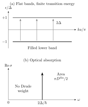
In this fixed-orbital model, both bands have zero group velocity but a nonzero interband current matrix element. At zero temperature the filled lower band absorbs at $\hbar\omega=2\Delta$. The arrow represents a delta function, not a finite-height peak; its positive-frequency area is $\pi D^{\mathrm{dia}}/2$. The contact and static interband terms cancel the zero-frequency pole.

Drude weight, sum rules and limit order

For a longitudinal component, write a possible dissipationless term as

$$\begin{aligned} \sigma_{aa}(z)&=\frac{iD^{\mathrm{Drude}}_{aa}}z +\sigma^{\mathrm{reg}}_{aa}(z),\\ \operatorname{Re}\sigma_{aa}(\omega) &=\pi D^{\mathrm{Drude}}_{aa}\delta(\omega) +\operatorname{Re}\sigma^{\mathrm{reg}}_{aa}(\omega). \end{aligned}$$

This defines the normalization of $D^{\mathrm{Drude}}$. It is the pole residue in the uniform optical response. It is not generally equal to $D^{\mathrm{dia}}$: virtual interband transitions and many-body correlations can transfer weight out of the pole. When the remaining kernel is regular at zero frequency, its residue is $D^{\mathrm{dia}}-\lim_{z\to0}\Pi(z)$ in that optical order of limits.

For the complete, consistently gauged model, the longitudinal optical sum rule is

$$\int_0^\infty d\omega\, \operatorname{Re}\sigma_{aa}(\omega) =\frac\pi2D^{\mathrm{dia}}_{aa}.$$

The integral includes half the weight of a delta function at the origin. This follows from the model’s causal high-frequency response and is one application of Sum Rules; Maldague (1977) derives the lattice kinetic-energy version. For the full nonrelativistic continuum electron model the weight is $\pi ne^2/(2m)$ with the bare electron mass. A restricted band model has its own contact term and omits higher-energy transitions; its partial sum is not automatically the continuum sum with an experimentally fitted effective mass.

Different response experiments take different limits. Write the probe wavevector as $\mathbf Q$ to distinguish it from carrier charge $q$.

Target	Limit or boundary condition	Physical question
Uniform optical response	$\mathbf Q=0$ before $\omega\to0$	Does a uniform field leave a persistent current?
Static longitudinal response	$\omega=0$ before $\mathbf Q\to0$	Does a pure gauge cancel from the bulk current?
Magnetic screening	Static transverse field, then $\mathbf Q\to0$	Is there a Meissner response?

A pure gauge produces no equilibrium bulk current in a simply connected region when states, boundaries and observables are transformed consistently. A constant vector potential on a periodic ring can instead encode a nonremovable boundary twist. Its energy curvature measures a stiffness; it is not a counterexample to local gauge invariance. Likewise, a clean normal metal can have a Drude delta without a Meissner effect. The optical and static transverse limits need not commute.

For a finite isolated sample, the spectrum is discrete. A smooth dissipative bulk dc coefficient ordinarily requires the thermodynamic limit and an identified relaxation mechanism before taking the dc limit. Integrability, momentum conservation or superconductivity can leave a delta function even after the thermodynamic limit. Transport Coefficients treats this classification; Drude Theory supplies the relaxation-time benchmark.

Interactions, disorder and conservation

The physical current vertices and contact term must be derived from the same Hamiltonian used for propagation. Charge conservation relates density and current response through continuity; its vertex identities are often called Ward identities. At finite $\mathbf Q$, the induced charge density and current must obey

$$-i\omega\,\delta\rho+i\mathbf Q\cdot\delta\mathbf j=0.$$

On a lattice this is the corresponding discrete divergence identity. Checking only the uniform optical spectrum cannot establish the full identity.

Replacing independent-electron propagators by dressed Green functions in a bare current bubble is an additional approximation. The self-energy and response vertex must be consistent if conservation is to be preserved. Baym and Kadanoff (1961) construct approximations in which the response follows from the same source-dependent propagator and satisfies the associated conservation constraints. Some models or symmetry limits simplify the vertex; the simplification must be demonstrated for the response being computed. Self-consistency of a one-particle calculation alone does not justify omitting its response vertex.

Disorder illustrates the physical issue. Forward scattering may strongly broaden a one-particle spectral peak while barely relaxing current. The transport lifetime can therefore differ greatly from the spectral lifetime. Impurity vertex corrections contain this directional information. Boltzmann Transport gives the collision-operator limit in which the distinction can be resolved semiclassically.

Numerical broadening also needs a physical interpretation. Replacing $\hbar\omega+i0^+$ by $\hbar\omega+i\eta$ uses an energy width $\eta$. It can make a finite spectrum readable. It does not, by itself, derive a transport lifetime or a finite dc resistivity. A relaxation model uses a rate $\gamma$ with $\eta=\hbar\gamma$ only when that identification follows from the chosen approximation. Converge size or momentum mesh, frequency resolution and broadening separately, and check whether a reported dc value survives the intended order of limits.

Hall and heat currents

The off-diagonal kernel uses products $v^a_{nm}v^b_{mn}$, including their complex phases. Replacing them by absolute squares loses the antisymmetric response. Tensor index order and the inherited Berry convention then determine the Hall sign; Hall Effect explains the signed tensor and its mechanisms. A longitudinal absorption formula cannot determine a Hall coefficient.

For thermal response, first identify a local energy density and derive its current from the same Hamiltonian’s energy continuity equation. For a conserved particle number and a common chemical potential,

$$\mathbf J_Q=\mathbf J_E-\mu\mathbf J_N,$$

where $\mathbf J_N$ transports particles and $\mathbf J_E$ transports energy. The subtraction uses number current, not charge current; for a single species $\mathbf J_q=q\mathbf J_N$. Interaction energy and the chosen energy-density assignment enter the energy-current construction. Substituting a band energy times a velocity without deriving that operator need not be valid in an interacting model.

Heat-current correlators are also not automatically thermal transport coefficients. Equilibrium circulating magnetization currents must be separated from currents carrying energy between reservoirs. Qin, Niu and Shi (2011) show how energy magnetization corrects thermal Hall response and restores the appropriate low-temperature Wiedemann–Franz relation in their noninteracting example. Thermoelectric Response develops the coupled charge/heat coefficient problem. The present electric-field response is not a derivation of a temperature-gradient source.

The parabolic Drude pole and the flat-band insulator provide complementary checks of a calculation: the first needs a contact term even with a vanishing current commutator; the second needs interband current matrix elements even with flat energies. Their integrated weights alone would not distinguish them. Resolving where the weight lies, with the correct delta/regular decomposition, tests information beyond the sum rule. Electronic Structure Methods Overview explains why a converged band calculation alone does not establish an accurate response.

Exercises

A lattice Drude weight

For a spinless one-dimensional band $\epsilon(k)=-2t\cos(ka)$ with $t>0$, fill $-k_F<k<k_F$ at zero temperature. Use length normalization and the thermodynamic limit to find $D^{\mathrm{dia}}$. Determine the low-density limit and the fully filled-band limit.

Solution

The current is diagonal in $k$ and commutes with this clean noninteracting Hamiltonian, so the uniform $\Pi$ vanishes. The contact term is

$$\begin{aligned} D^{\mathrm{dia}}&=\frac{q^2}{\hbar^2} \int_{-k_F}^{k_F}\frac{dk}{2\pi}\,2ta^2\cos(ka)\\ &=\frac{2q^2ta}{\pi\hbar^2}\sin(k_Fa) =\frac{q^2v_F}{\pi\hbar}. \end{aligned}$$

It equals $D^{\mathrm{Drude}}$ for this model. At low density, $n_{1\mathrm D}=k_F/\pi$ and $m^*=\hbar^2/(2ta^2)$ give $D=n_{1\mathrm D}q^2/m^*$. At full filling $k_Fa=\pi$, the curvature integrates to zero and the band cannot carry a Drude current. Adding a spin degeneracy would double the result only if both spin bands had this same filling.

Where the flat-band spectral weight goes

For the two-orbital model in the text, calculate $\partial_k^2h$, $\Pi(0)$ and the positive-frequency integrated absorption. Explain what fails if the Hamiltonian is diagonalized first and its diagonal eigenvalues alone are differentiated.

Solution

Since $\partial_k^2h=-a^2h$, each occupied lower-band state contributes $a^2\Delta$ to its expectation value. Thus $D^{\mathrm{dia}}=q^2\Delta a/\hbar^2$. The two directed interband terms give

$$\Pi(z)={}\frac{q^2N}{L}\frac{\Delta^2a^2}{\hbar^2} \times\left[\frac1{\hbar z+2\Delta}-\frac1{\hbar z-2\Delta}\right].$$

At $z=0$ this is exactly $D^{\mathrm{dia}}$, so the Drude residue is zero. For $\omega>0$ only the lower-to-upper transition absorbs:

$$\begin{aligned} \int_0^\infty d\omega\,\operatorname{Re}\sigma(\omega) &=\frac{\pi q^2N}{L}\frac{\Delta^2a^2}{\hbar^2} \frac1{2\Delta}\\ &=\frac\pi2D^{\mathrm{dia}}. \end{aligned}$$

The identity $\int_0^\infty d\omega\,\delta(\hbar\omega-2\Delta)/\omega=1/(2\Delta)$ includes the energy-to-frequency Jacobian. The current transformed into the eigenbasis has nonzero off-diagonal entries. Differentiating the constant diagonal energies instead would remove these entries and the entire absorption line.

Broadening and a false dc conclusion

Let $\sigma(\omega)=D/(\gamma-i\omega)$ with $D>0$ and $\gamma>0$. Find its real part, dc value and positive-frequency integrated weight. What can be inferred if a finite-spectrum calculation changes its apparent dc value when its artificial broadening is halved?

Solution

$$\begin{aligned} \operatorname{Re}\sigma(\omega)&=\frac{D\gamma}{\gamma^2+\omega^2},\\ \sigma(0)&=\frac D\gamma,\\ \int_0^\infty d\omega\,\operatorname{Re}\sigma&=\frac{\pi D}{2}. \end{aligned}$$

The peak height diverges as $\gamma\to0$, while its weight is unchanged; distributionally it tends to $\pi D\delta(\omega)$. A broadening-dependent height can represent unresolved ballistic weight or discrete levels. It does not establish a material resistivity. One must identify a physical relaxation approximation and test the size, resolution and dc limits before assigning $\gamma$ to a transport rate.

A missing-contact diagnostic

A program correctly obtains $\Pi=0$ for the uniform current of a clean parabolic electron gas, then reports zero conductivity. Identify the omitted term. Would requiring every static uniform vector potential to cancel also be a valid test on a periodic ring?

Solution

It omitted $D^{\mathrm{dia}}=ne^2/m$, the expectation of the Hamiltonian’s second derivative with respect to the vector potential. The correct optical response is $ine^2/[m(\omega+i0^+)]$ with a Drude delta. The same operator’s field dependence supplies the contact current; a vanishing commutator does not imply a vanishing response to the electric field.

A ring requires a separate boundary-condition check. A uniform vector potential generally changes its flux twist and is not removable by a single-valued gauge transformation. Pure-gauge cancellation in a simply connected bulk, optical stiffness and flux sensitivity are distinct tests.

References

• Baym, Gordon, and Leo P. Kadanoff. “Conservation Laws and Correlation Functions.” Physical Review 124, 287–299 (1961). doi:10.1103/PhysRev.124.287. Conserving approximations and the connection between propagation, vertices and response constraints.
• Kubo, Ryogo. “Statistical-Mechanical Theory of Irreversible Processes. I. General Theory and Simple Applications to Magnetic and Conduction Problems.” Journal of the Physical Society of Japan 12, 570–586 (1957). doi:10.1143/JPSJ.12.570. The linear-response framework used by the canonical Kubo derivation.
• Maldague, Pierre F. “Optical Spectrum of a Hubbard Chain.” Physical Review B 16, 2437–2446 (1977). doi:10.1103/PhysRevB.16.2437. Lattice electromagnetic coupling, current response and the kinetic-energy optical sum rule.
• Qin, Tao, Qian Niu, and Junren Shi. “Energy Magnetization and the Thermal Hall Effect.” Physical Review Letters 107, 236601 (2011). doi:10.1103/PhysRevLett.107.236601; arXiv:1108.3879. Energy magnetization corrections to thermal transport.