Polarons in Materials

A lattice polaron is an electronic carrier together with the ionic response that dresses its motion. In a material, calling a carrier a polaron is useful only when the proposed lattice coupling accounts for observable changes relative to a specified electronic reference. A heavy band, a broad spectral satellite or an activated conductivity alone does not determine the dressing mechanism.

This page connects generic dressing theory to dilute electron or hole carriers in a stable lattice. It distinguishes the spatial size of the distortion, the energy gained by relaxation, the coherence of motion and the temperature dependence of transport. Finite carrier density, disorder, multiple bands and a dielectric environment can change all four. The general mobile-impurity construction and its displacement transformations remain with Polarons Preview; Fermi polarons and carriers dressed primarily by spin excitations are outside this material specialization.

Required background. Polarons Preview supplies energy, mass, residue, conditional clouds and the generic Fröhlich/Holstein benchmarks. Electron–Phonon Coupling supplies normalized material vertices, reference bands and the distinction between a model interaction and a screened first-principles input.

Helpful background. Spectral Functions supplies poles and probe-dependent line shapes; Effective Mass distinguishes curvature and measured masses. Boltzmann Transport supplies the assumptions behind coherent quasiparticle kinetics, and Optical Conductivity supplies spectral-weight accounting.

Carrier and lattice energy scales

Start with an electronic dispersion at a specified reference structure and with a declared treatment of electronic correlations. Its curvature mass $m_b$ is the input to a subsequent lattice-dressing calculation. A mass measured after that dressing is generally an output. Reusing it as $m_b$ can count the same interaction twice.

For a hole, use the positive low-energy hole dispersion obtained from the chosen valence band. Neither the free-electron mass nor an electron–hole reduced mass can replace the carrier’s band mass without changing the problem. Nearly degenerate bands, valleys or orbitals may require a matrix Hamiltonian rather than one scalar mass.

The other inputs are the stable phonon energies $\varepsilon_{\mathbf q\nu}=\hbar\omega_{\mathbf q\nu}$, their eigenvectors and coupling vertices, the spatial extent of those vertices, and the screening appropriate to the carrier density and geometry. The lattice spacing $a$, reference bandwidth $W$, carrier concentration, temperature and disorder scale set the regime. Here $W$ is the full bandwidth and $D_0=W/2$ its half-width.

These inputs answer different questions. Comparing a lattice relaxation energy with $D_0$ tests the competition with electronic delocalization. Comparing a phonon energy with $D_0$ tests whether ionic motion is slow or fast relative to the electronic band scale. Comparing the resulting coherent bandwidth with scattering and temperature scales tests whether a band-transport description remains useful. No single dimensionless number replaces this sequence.

Three-dimensional polar coupling

For an isotropic parabolic carrier band coupled to one dispersionless longitudinal-optical mode in a three-dimensional insulating host, define

$$\begin{aligned} \alpha&=\frac{e^2}{4\pi\epsilon_0\hbar} \sqrt{\frac{m_b}{2\varepsilon_{\rm LO}}} \left(\frac1{\epsilon_\infty}-\frac1{\epsilon_s}\right),\\ \ell_{\rm LO}&=\frac{\hbar}{\sqrt{2m_b\varepsilon_{\rm LO}}}. \end{aligned}$$

Here $e>0$, $\epsilon_0$ is the vacuum permittivity, and $\epsilon_\infty,\epsilon_s$ are relative dielectric constants of the host: electronic screening above the relevant lattice resonances, and static screening including them. Free-carrier screening is absent from this elementary Fröhlich reduction. A multibranch polar crystal requires mode-resolved couplings; it need not admit one representative LO frequency.

The inverse-dielectric difference isolates the additional ionic polarization. If $\epsilon_s=\epsilon_\infty$, this coupling vanishes. At fixed $\epsilon_\infty$, sending $\epsilon_s$ to infinity gives a finite limit, not infinite coupling. The recoil length $\ell_{\rm LO}$ compares kinetic and phonon energies; it is not a measured cloud radius. A continuum approximation must still be tested against the momenta actually sampled and the lattice spacing.

The generic three-dimensional weak-coupling result gives

$$\begin{aligned} \Delta E&=-\alpha\varepsilon_{\rm LO} +O(\alpha^2\varepsilon_{\rm LO}),\\ \frac{m_{\rm pol}}{m_b}&=1+\frac{\alpha}{6}+O(\alpha^2). \end{aligned}$$

These are useful input and unit checks for small $\alpha$. They are not formulas for an arbitrary optical spectrum, nor a license to extrapolate a first-order mass correction to strong coupling. Devreese and Alexandrov review how the continuum model and its response change beyond these limits.

In a monolayer or an interface, the electric field extends outside the carrier’s layer. Thickness, dielectric boundaries, remote substrate modes and gates alter the momentum dependence of the vertex, as treated explicitly by Sio and Giustino. One cannot obtain a material two-dimensional polaron by changing only the integration dimension in the bulk formula. Use Two-Dimensional Materials and Dielectric Response to specify that electrostatic problem before making a polaron reduction.

Local relaxation and hopping modulation

For the single-carrier Holstein convention $g n_i(b_i+b_i^\dagger)$, with phonon energy $\varepsilon_{\rm ph}$ and energy-unit $g$, the generic displaced-oscillator result supplies

$$E_p=\frac{g^2}{\varepsilon_{\rm ph}}, \qquad S=\left(\frac{g}{\varepsilon_{\rm ph}}\right)^2 =\frac{E_p}{\varepsilon_{\rm ph}}.$$

$E_p>0$ is the atomic relaxation-energy magnitude; the energy change is $-E_p$. The independent material ratios may be taken as $E_p/D_0$ and $\varepsilon_{\rm ph}/D_0$; their quotient is $S$. Two materials with the same relaxation energy and bandwidth can have different oscillator overlaps because their phonon energies differ.

In a small-hopping, low-temperature expansion about independent local oscillators, the leading coherent transfer is

$$t_{\rm coh}=t e^{-S}.$$

This is the ground-state oscillator-overlap contribution, not an exact finite-temperature bandwidth or a universal mobility formula. Its derivation belongs to the Holstein benchmark. Corrections, other phonon branches and nonlocal coupling must be checked before using it quantitatively.

When displacement primarily modulates transfer between orbitals, a Peierls or SSH-type vertex is more appropriate than a local density vertex. The distortion can then change the shape and minimum of the band, not merely multiply every hopping by the Holstein overlap. The SSH model studied by Marchand and collaborators has a coupling-driven change in ground-state momentum. This is a useful counterexample to the claim that every single-polaron evolution must be a smooth crossover.

Distortion size and translational motion

“Large” and “small” describe the spatial organization of the carrier–lattice correlation relative to the crystal. They do not directly label conductivity. A locally correlated small polaron can propagate coherently through a narrow Bloch band; a spatially extended cloud can coexist with poor transport caused by disorder or other scattering.

In a clean one-carrier momentum eigenstate, the one-point carrier density is spread over the crystal. Its lattice cloud can nevertheless be local. For site occupation $n_0$ and a displacement component $u_j$, a useful diagnostic is

$$C_j=\frac{\langle n_0u_j\rangle}{\langle n_0\rangle} -\langle u_j\rangle.$$

This is the excess displacement conditioned on finding the carrier at the origin, relative to the unconditional mean. State which displacement component, polarization or energy-weighted measure defines a reported radius. Sign-changing clouds and long tails make an unspecified “polaron size” ambiguous.

A localized electronic state with a relaxed ionic distortion is an informative variational or adiabatic configuration. Equivalent translated configurations may hybridize into translational eigenstates. A static symmetry-broken calculation therefore does not, by itself, establish an immobile exact quantum ground state or a thermodynamic localization transition. Defects can pin such a configuration, but pinning is an additional physical ingredient.

At finite concentration, cloud overlap, Pauli filling, carrier screening and carrier–carrier interactions can invalidate the single-polaron picture. A density-dependent spectrum must be compared at the same structure and screening conditions. Dividing a many-carrier optical mass by a bare band mass is not automatically a measurement of the isolated-polaron mass.

Coherent motion and thermally assisted hopping

In a coherent regime, a dispersing spectral feature can support a wave-packet and collision description. One must resolve its dispersion and width and identify a mechanism that relaxes current. Even in a scalar isotropic approximation, $\mu=e\tau_{\rm tr}/m_{\rm pol}$ requires a transport relaxation time. The electron spectral lifetime is not generally that time. The general collision and current-vertex derivations are in Boltzmann Transport and Kubo Formula in Materials.

In an incoherent hopping regime, the useful variables are populations of locally relaxed configurations and transition rates between them. Such a reduction requires loss of phase coherence and equilibration assumptions; a finite isolated oscillator with a discrete spectrum does not alone provide an irreversible rate. Temperature can promote this regime, but there is no universal transition at $k_{\rm B}T=\varepsilon_{\rm ph}$.

Reorganization energy and the hopping barrier

Consider equivalent left and right sites whose effective classical distortion coordinate is $Q$. Equal-curvature diabatic surfaces, each referred to its own minimum energy, are

$$\begin{aligned} U_L(Q)&=\frac K2(Q+Q_0)^2,\\ U_R(Q)&=\frac K2(Q-Q_0)^2,\\ \lambda_{\rm r}&=2KQ_0^2. \end{aligned}$$

“Diabatic” means the electronic carrier is assigned to one site while the ions move. The energy to move the carrier vertically from $L$ to $R$ at $Q=-Q_0$, before the ions relax, is $\lambda_{\rm r}$. The surfaces cross at $Q=0$, where their energy above either minimum is $\lambda_{\rm r}/4$.

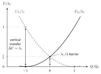
The two diabatic energies have equal minima and cross at one quarter of the reorganization energy. A vertical transfer at the left minimum costs $\lambda_{\rm r}$. These are potential-energy surfaces in a classical coordinate, not two stationary eigenstates of the full electron–phonon problem. Electronic mixing rounds their crossing.

For independent identical Holstein oscillators, a hop removes the old distortion and creates the new one. Their two relaxation costs add, giving $\lambda_{\rm r}=2E_p$. Thus the symmetric diabatic barrier is $E_p/2$, whereas the vertical transfer costs $2E_p$. Neither is the atomic energy lowering $-E_p$.

Finite electronic mixing changes the adiabatic barrier. Diagonalizing the symmetric two-state potential matrix with off-diagonal transfer $t$ gives

$$U_-(Q)=\frac K2(Q^2+Q_0^2) -\sqrt{K^2Q^2Q_0^2+|t|^2}.$$

Its two minima exist for $|t|<\lambda_{\rm r}/2$, and their barrier is $E_a^{\rm ad}=(\lambda_{\rm r}/2-|t|)^2/\lambda_{\rm r}$. At larger mixing the lower surface has a single minimum at the crossing coordinate. This classical surface change is not a quantum localization transition, and a barrier alone does not specify a dynamical hopping prefactor. The weak-transfer rate below instead uses the diabatic crossing and treats $t$ perturbatively.

An offset $\Delta G=U_R^{\min}-U_L^{\min}$ shifts the second surface upward. Solving $U_L(Q_c)=U_R(Q_c)$ gives

$$\begin{aligned} Q_c&=\frac{\Delta G}{2KQ_0},\\ E_{a,L\to R}&=\frac{(\lambda_{\rm r}+\Delta G)^2}{4\lambda_{\rm r}},\\ E_{a,R\to L}&=\frac{(\lambda_{\rm r}-\Delta G)^2}{4\lambda_{\rm r}}. \end{aligned}$$

The barrier difference is $\Delta G$, as detailed balance requires for equal statistical prefactors. This one-coordinate construction is an effective harmonic free-energy model when additional equilibrated coordinates have been integrated out.

In the weak electronic-transfer, classical harmonic-bath limit, the corresponding nonadiabatic rate to one specified neighbor is

$$w_{ij}=\frac{2\pi |t_{ij}|^2} {\hbar\sqrt{4\pi\lambda_{\rm r} k_{\rm B}T}} \exp\!\left[-\frac{(\lambda_{\rm r}+\Delta G)^2} {4\lambda_{\rm r} k_{\rm B}T}\right].$$

In the left thermal ensemble, the vertical energy gap is Gaussian with mean $\lambda_{\rm r}+\Delta G$ and variance $2\lambda_{\rm r}k_{\rm B}T$. Golden-rule sampling at zero gap gives the displayed factor $2\pi|t_{ij}|^2/\hbar$ times that Gaussian probability density. Its use requires thermally classical participating modes, equilibrated initial configurations and sufficient environmental broadening/dephasing for a rate description. Quantum high-frequency modes, anharmonic surfaces or strong electronic mixing require another calculation. Marcus and Sutin discuss this harmonic electron-transfer limit; Holstein’s work treats the lattice-polaron transport problem and its coherent versus hopping regimes.

For equivalent sites on an isotropic $d$-dimensional hypercubic lattice of spacing $a$, let $w$ be the rate to each of the $2d$ neighbors. The total escape rate is $2dw$ and the diffusion constant is

$$\begin{aligned} D_{\rm diff}&=a^2w,\\ \mu&=\frac{eD_{\rm diff}}{k_{\rm B}T},\\ \sigma&=ne\mu. \end{aligned}$$

The Einstein relation here assumes dilute nondegenerate carriers in equilibrium and linear response; $\mu$ is a positive mobility magnitude. Concentrated or disordered networks need their own occupation, correlation and connectivity factors. In particular, a conductivity activation energy can contain both a mobility barrier and the temperature dependence of $n$.

When neither limiting transport picture works

The small-hopping overlap and classical activated rate describe different limits. Interpolating them by adding their mobilities is not a derivation. Dynamical disorder in transfer integrals can interrupt coherent motion without producing the independent, fully relaxed hops assumed above. The transient-localization framework discussed by Fratini, Mayou and Ciuchi provides an example of this intermediate situation in molecular crystals.

Likewise, a negative temperature coefficient of mobility does not by itself prove a long-lived Bloch quasiparticle, and an approximately Arrhenius resistivity does not uniquely identify lattice polarons. Establish the electronic structure and carrier population, test the relevant time scales, and compare more than one observable.

Formation energies and measured response

Keep four energies distinct: the total energy change on dressing; an electronic eigenvalue in a fixed distorted structure; a vertical optical or removal energy; and a barrier along a transport path. They involve different final states and different opportunities for the ions to relax. The two-surface example makes the distinction explicit even before electronic correlations are added.

First-principles calculations supply bands, phonons, vertices and candidate distortions. Localized and extended solutions must be compared at the same charge and boundary conditions. Finite-cell effects and the treatment of electronic self-interaction can bias localization, while a charged-cell correction changes the formation-energy comparison. A relaxed distortion is meaningful only with its reference energy and stability specified.

The adiabatic formulation of Sio and collaborators distinguishes its total formation energy from the eigenvalue of the nonlinear electronic problem and treats the nuclei classically. Such an optimized distortion does not yet give a coherent bandwidth, finite-temperature mobility or quantum spectral residue. Zero-point motion and dynamical dressing must be included by methods appropriate to the requested output. Electronic Structure Methods Overview explains the different meanings of model, density-functional and quasiparticle energies.

Test the same model against different observables

Single-particle spectra. A reproducible satellite spacing, dispersion change and temperature dependence can constrain a phonon-dressing model. Spectral residue is an overlap with the chosen electronic creation operator, not a literal fraction of unbound electrons. Matrix elements, resolution, extrinsic losses, electronic correlations and other bosonic excitations can alter observed line shapes. Use Angle-Resolved Photoemission for the measurement model rather than identifying every replica with an intrinsic polaron satellite.

Optical weight. A model may transfer weight from a coherent response to phonon-assisted finite-frequency absorption. Test the conductivity with consistent carrier density, tensor direction, cutoff and electronic reference. A mid-infrared peak is not generally equal to $E_p$ or $2E_p$; the simple vertical value above belongs to its declared two-site limit. Interband absorption and other correlation effects can occupy the same window.

Lattice and isotope response. A carrier-correlated distortion and coupling-compatible phonon changes connect the electronic interpretation to the lattice. Isotope substitution changes frequencies and zero-point amplitudes together. For a local physical force $F$ and spring constant $K$, held fixed while the mass $M$ changes,

$$\begin{aligned} \omega&=\sqrt{K/M},& g&=F\sqrt{\frac{\hbar}{2M\omega}},\\ E_p&=\frac{F^2}{2K},& S&=\frac{F^2}{2K\hbar\omega}. \end{aligned}$$

In this harmonic idealization $E_p$ is mass-independent while $S\propto\sqrt M$. Holding the energy-unit $g$ fixed during the same isotope substitution would describe a different model. Real structural and anharmonic isotope changes must be assessed separately.

Transport. Determine whether measured activation comes from carrier release, hopping, contacts, percolation or a combination. A Hall density need not equal the population entering a hopping model without a Hall theory for that regime. Compare transport and optical constraints rather than using a single fitted mass or barrier to explain every measurement.

The strongest inference is a common model with independently constrained inputs and successful predictions across these channels. A fit to one curve can establish compatibility; it cannot uniquely identify the microscopic mechanism. A bipolaron or a superconducting instability is an additional many-carrier claim requiring interaction, statistics and stability analysis.

Exercises

1. Check the scales of a bulk polar model

A hypothetical isotropic bulk model has $m_b=0.20m_e$, $\varepsilon_{\rm LO}=60\,\mathrm{meV}$, $\epsilon_\infty=10$, $\epsilon_s=12$ and $a=0.40\,\mathrm{nm}$. Calculate $\alpha$, the leading weak-coupling energy and mass corrections, and $\ell_{\rm LO}/a$. Then change only $\epsilon_s$ to 24 and find the change in $\alpha$. Does $\alpha$ diverge if $\epsilon_s$ tends to infinity with every other input fixed?

Solution

Using SI inputs and converting the phonon energy to joules gives

$$\begin{aligned} \alpha&=0.11224,\\ \Delta E&\simeq-6.7344\,\mathrm{meV},\\ m_{\rm pol}/m_b&\simeq1.01871,\\ \ell_{\rm LO}&=1.78185\,\mathrm{nm}\simeq4.45a. \end{aligned}$$

The energy and mass numbers are leading-order model estimates. The length comparison does not measure a cloud radius or establish asymptotically exact continuum behavior; relevant momenta must also remain small compared with reciprocal-lattice scales.

The inverse-dielectric difference changes from $1/60$ to $7/120$, multiplying $\alpha$ by 3.5. Thus the new coupling is 0.39284. In the stated mathematical limit,

$$\alpha_{\epsilon_s\to\infty}=0.67344.$$

The finite limit follows from $1/\epsilon_s\to0$. A real material need not allow its static dielectric response to vary while its phonons, mass and electronic dielectric response remain fixed. In particular, a conducting dc response is not the insulating-host $\epsilon_s$ assumed here.

2. Equal relaxation energies, unequal coherent bands

Two one-dimensional Holstein models have nearest-neighbor transfer $t=2\,\mathrm{meV}$ and atomic relaxation energy $E_p=80\,\mathrm{meV}$. Their phonon energies are 20 and $80\,\mathrm{meV}$. Find $g$, $S$, $E_p/D_0$ and $\varepsilon_{\rm ph}/D_0$ for each. Estimate their leading coherent bandwidths in the small-hopping, zero-temperature projection. Why does their equality of $E_p$ not imply equal narrowing?

Solution

The reference chain has $W=4t=8\,\mathrm{meV}$ and $D_0=4\,\mathrm{meV}$. For the two models, labeled A and B,

$$\begin{aligned} g_A&=\sqrt{80\cdot20}\,\mathrm{meV}=40\,\mathrm{meV},\\ g_B&=\sqrt{80\cdot80}\,\mathrm{meV}=80\,\mathrm{meV},\\ S_A&=4,\qquad S_B=1. \end{aligned}$$

Both have $E_p/D_0=20$, whereas $\varepsilon_{\rm ph}/D_0$ is 5 and 20. The first-order band estimates are

$$\begin{aligned} W_{{\rm coh},A}&=8e^{-4}\,\mathrm{meV}\simeq0.14653\,\mathrm{meV},\\ W_{{\rm coh},B}&=8e^{-1}\,\mathrm{meV}\simeq2.9430\,\mathrm{meV}. \end{aligned}$$

Their ratio is $e^3\simeq20.09$. The relevant overlap depends on the displacement in oscillator units, $S=E_p/\varepsilon_{\rm ph}$, not on $E_p$ alone. The small ratios $t/\varepsilon_{\rm ph}=0.1$ and 0.025 motivate the leading projection; finite-hopping corrections still require an error estimate. Neither bandwidth is a calculated mobility.

3. Relaxation, vertical transfer and activation

Take two independent classical coordinates $q_1,q_2$ with spring constant $K=4\,\mathrm{eV/\mathring A^2}$ and a carrier force $F>0$. The electronic carrier occupies site 1 or 2:

$$\begin{aligned} U_1&=\frac K2(q_1^2+q_2^2)-Fq_1,\\ U_2&=\frac K2(q_1^2+q_2^2)-Fq_2. \end{aligned}$$

Choose $F$ so that the atomic relaxation energy is $120\,\mathrm{meV}$. Find the relaxed displacement, the vertical transfer cost and the symmetric crossing barrier. Raise the minimum of site 2 by $\Delta G=30\,\mathrm{meV}$ and calculate both directed barriers. As a separate classical-bath estimate, use equivalent sites, $t_{12}=2\,\mathrm{meV}$, $T=300\,\mathrm K$ and $a=0.4\,\mathrm{nm}$ to calculate the per-neighbor rate and positive mobility. Assume the participating bath modes are classical and equilibrate between hops.

Solution

Completing each quadratic gives $E_p=F^2/(2K)$ and $q_*=F/K$. Numerically,

$$\begin{aligned} F&=0.97980\,\mathrm{eV/\mathring A},\\ q_*&=0.24495\,\mathring A. \end{aligned}$$

The two minima are $(q_*,0)$ and $(0,q_*)$, each with energy $-E_p$. A vertical transfer from the first geometry changes the energy from $-E_p$ to $+E_p$, so $\lambda_{\rm r}=2E_p=240\,\mathrm{meV}$. Minimizing the common energy on the crossing line $q_1=q_2$ gives $q_1=q_2=q_*/2$ and

$$E_a=\frac{\lambda_{\rm r}}4=60\,\mathrm{meV}.$$

The detuned barriers are

$$\begin{aligned} E_{a,1\to2}&=\frac{(240+30)^2}{4\cdot240}\,\mathrm{meV} \\ &=75.9375\,\mathrm{meV},\\ E_{a,2\to1}&=\frac{(240-30)^2}{4\cdot240}\,\mathrm{meV} \\ &=45.9375\,\mathrm{meV}. \end{aligned}$$

Their difference is the required $30\,\mathrm{meV}$. With equal prefactors, $w_{1\to2}/w_{2\to1}=\exp[-\Delta G/(k_{\rm B}T)]$.

For the separate equivalent-site transport estimate, $k_{\rm B}T=25.852\,\mathrm{meV}$ and $\hbar=0.658212\,\mathrm{meV\,ps}$. Substitution gives

$$\begin{aligned} w&=0.0134264\,\mathrm{ps}^{-1},\\ D_{\rm diff}&=2.14823\times10^{-9}\,\mathrm{m^2\,s^{-1}},\\ \mu&=8.3097\times10^{-4}\,\mathrm{cm^2\,V^{-1}\,s^{-1}}. \end{aligned}$$

$w$ is the rate to one neighbor. Inserting the total escape rate directly into $D_{\rm diff}=a^2w$ would overcount by $2d$. These numbers illustrate the explicitly assumed classical harmonic bath; the static two-coordinate surfaces alone do not establish its dynamical validity.

4. What an Arrhenius plot actually measures

In a hypothetical fixed-parameter classical nonadiabatic hopping model, the mobility barrier is $E_a=60\,\mathrm{meV}$, and the carrier population has an additional activation $n(T)=n_0\exp[-E_d/(k_{\rm B}T)]$ with $E_d=20\,\mathrm{meV}$. Derive $\sigma(T)$ up to a temperature-independent constant. Find the local raw Arrhenius slope

$$E_{\rm slope}(T)=-k_{\rm B}\frac{d\ln\sigma}{d(1/T)}$$

at 300 K. Which energy is obtained after removing the predicted temperature prefactor?

Solution

The classical nonadiabatic rate contains $T^{-1/2}$ and the Einstein relation contributes another $T^{-1}$. Consequently,

$$\sigma(T)\propto T^{-3/2} \exp\!\left[-\frac{E_a+E_d}{k_{\rm B}T}\right].$$

Writing $x=1/T$ gives $\ln\sigma=\text{constant}+(3/2)\ln x-(E_a+E_d)x/k_{\rm B}$, and hence

$$\begin{aligned} E_{\rm slope}(T)&=E_a+E_d-\frac32 k_{\rm B}T,\\ E_{\rm slope}(300\,\mathrm K)&=41.2220\,\mathrm{meV}. \end{aligned}$$

Fixed reference units inside each logarithm are implicit and do not affect these derivatives. A plot of $\ln[\sigma T^{3/2}]$ against $1/T$ removes this model’s prefactor and gives $80\,\mathrm{meV}$. That still includes carrier activation; recovering the $60\,\mathrm{meV}$ mobility barrier requires independent information about $n(T)$. Neither slope is the $120\,\mathrm{meV}$ atomic relaxation energy of the preceding exercise.

An adiabatic attempt-rate model, variable-range hopping or a changing electronic structure need not have this prefactor. Straightening a curve by choosing a power of $T$ does not establish the model.

References

• J. T. Devreese and A. S. Alexandrov, “Fröhlich polaron and bipolaron: Recent developments,” Reports on Progress in Physics 72, 066501 (2009), doi:10.1088/0034-4885/72/6/066501. Continuum and lattice regimes, response and the limits of simple mass or hopping estimates.
• S. Fratini, D. Mayou and S. Ciuchi, “The transient localization scenario for charge transport in crystalline organic materials,” Advanced Functional Materials 26, 2292–2315 (2016), doi:10.1002/adfm.201502386. Dynamical-disorder transport beyond a simple band-versus-independent-hop dichotomy.
• T. Holstein, “Studies of polaron motion: Part I. The molecular-crystal model,” Annals of Physics 8, 325–342 (1959), doi:10.1016/0003-4916(59)90002-8; “Part II. The ‘small’ polaron,” 8, 343–389 (1959), doi:10.1016/0003-4916(59)90003-X. Local electron–lattice models and the distinction between coherent and hopping motion.
• D. J. J. Marchand, G. De Filippis, V. Cataudella, M. Berciu, N. Nagaosa, N. V. Prokof’ev, A. S. Mishchenko and P. C. E. Stamp, “Sharp Transition for Single Polarons in the One-Dimensional Su-Schrieffer-Heeger Model,” Physical Review Letters 105, 266605 (2010), doi:10.1103/PhysRevLett.105.266605. A bounded counterexample to a universal smooth-crossover claim.
• R. A. Marcus and N. Sutin, “Electron transfers in chemistry and biology,” Biochimica et Biophysica Acta — Reviews on Bioenergetics 811, 265–322 (1985), doi:10.1016/0304-4173(85)90014-X. Harmonic reorganization surfaces, detailed balance and weak-transfer classical rate theory.
• W. H. Sio and F. Giustino, “Unified ab initio description of Fröhlich electron-phonon interactions in two-dimensional and three-dimensional materials,” Physical Review B 105, 115414 (2022), doi:10.1103/PhysRevB.105.115414. Geometry and dielectric environment in the long-range vertex.
• W. H. Sio, C. Verdi, S. Poncé and F. Giustino, “Ab initio theory of polarons: Formalism and applications,” Physical Review B 99, 235139 (2019), doi:10.1103/PhysRevB.99.235139. First-principles material inputs, total formation energies and the scope of adiabatic localized solutions.