Two-Dimensional Materials

A two-dimensional material is a crystalline sheet whose electronically and mechanically relevant thickness is one or a few atomic layers. Its carriers may be kinematically two dimensional, but its electric fields, photons, substrate modes, and contacts generally inhabit a three-dimensional environment. That mixed-dimensional character is responsible for much of the subject’s distinctive physics.

The phrase names a platform class, not one band structure or phase. Graphene is a gapless Dirac semimetal; hexagonal boron nitride is a wide-gap insulator; many transition-metal dichalcogenide monolayers are semiconductors; other layered compounds can be metallic, magnetic, ferroelectric, or superconducting. Layer count, stacking, strain, encapsulation, dielectric environment, contacts, and gate configuration can all change the measured system.

Required background. Low-Dimensional Quantum Matter supplies the distinction between a thin structure and low-dimensional dynamics. Band Theory Overview supplies band, filling and gap terminology. Random Phase Approximation supplies the self-consistent density-response framework needed to distinguish a bare electrostatic interaction from a screened one.

Atomically thin crystals and material observables

An atomically thin crystal is different from an interface-confined electron gas: the former is the material itself, while the latter is a population of carriers inside a thicker host. We will follow how thinning changes a crystal, how its surroundings screen charges, and how optical and electrical measurements probe the resulting system.

Layered bonding creates an exfoliation plane

Many atomically thin crystals descend from three-dimensional parent compounds with strong in-plane bonding and weaker interlayer adhesion. Mechanical or liquid exfoliation separates layers; chemical vapor deposition, epitaxy, and other growth methods can instead form sheets directly. “Van der Waals material” usually describes the weakly bonded stacking direction, not the absence of covalent or ionic bonds inside a layer.

A monolayer may contain more than one atomic plane. Monolayer MoS₂, for example, is an S–Mo–S trilayer in atomic structure but one electronically coherent layer. The physically relevant layer count must therefore be tied to a crystallographic repeat unit, not to a casual count of visible planes.

For specific examples, Graphene explains a semimetal, Transition-Metal Dichalcogenides develops semiconducting and metallic layers, and 2D Magnets and Ferroelectrics treats ordered layers. These are different Hamiltonians, not interchangeable realizations of one universal two-dimensional phase.

A crystal can be flat without being perfectly planar

For an elastic membrane with out-of-plane displacement $h(\mathbf r)$, a harmonic free energy contains bending and tension,

$$F_h = \frac{1}{2} \int d^2r\, \left[ \kappa_b(\nabla^2h)^2 + \sigma|\nabla h|^2 \right],$$

where $\kappa_b$ is bending rigidity and $\sigma$ is tension. With areal mass density $\rho_{2D}$, the flexural dispersion is

$$\omega_{\mathrm{ZA}}^2(q) = \frac{\kappa_bq^4+\sigma q^2}{\rho_{2D}}.$$

Use $h_{\mathbf q}=A^{-1}\int_A d^2r\,h(\mathbf r)e^{-i\mathbf q\cdot\mathbf r}$ for area $A$. In the classical thermal regime, a tensionless harmonic membrane has

$$\left\langle |h_{\mathbf q}|^2\right\rangle = \frac{k_BT}{A\kappa_bq^4},$$

which is strongly infrared sensitive. This does not imply that atomically thin crystals cannot exist. In a crystalline membrane, nonlinear coupling between bending and in-plane strain renormalizes the long-wavelength elasticity; finite size, tension, substrate pinning, and microscopic corrugation also matter. Suspended graphene is experimentally corrugated rather than an ideal mathematical plane.

A crystal constrained to an exact plane and a flexible sheet embedded in three dimensions are different statistical-mechanical models. Do not transfer a statement about translational correlations in the former directly to the latter. Nelson and Peliti (1987) show why bending and stretching must be treated together; Meyer and collaborators (2007) observed corrugations in suspended graphene. Neither a divergent harmonic height variance nor a microscopic ripple alone determines a real membrane’s stability.

Removing a layer can change the band structure

Layer reduction changes more than confinement energy. It can remove inversion symmetry, alter orbital hybridization, change dielectric self-energy, and move different valleys by unequal amounts. A familiar example is the indirect-to-direct optical crossover of MoS₂ at monolayer thickness. The conclusion is material specific: monolayer formation does not generically make a semiconductor direct gap.

Mak and collaborators (2010) observed the direct-gap optical behavior of monolayer MoS₂. A quoted gap still needs its measurement specified: a neutral optical resonance is not the energy for adding and removing charged particles. The distinction is developed below.

Charges are screened by the sheet and its surroundings

Fields escape the sheet

In a bulk isotropic insulator, long-wavelength electrostatics is often summarized by one dielectric constant. In an atomically thin layer, electric field lines extend into the media above and below the sheet. Screening is therefore nonlocal and environmentally tunable.

For an isotropic polarizable sheet between media with relative permittivities $\epsilon_t$ and $\epsilon_b$, define

$$\kappa_{\mathrm{env}} = \frac{\epsilon_t+\epsilon_b}{2}.$$

We use the two-dimensional Fourier convention $V(\mathbf r)=\int d^2q\,e^{i\mathbf q\cdot\mathbf r}V(q)/(2\pi)^2$. Thus $V(r)$ has units of energy and $V(q)$ has units of energy times area. For charges of magnitude $e$, the repulsive Rytova–Keldysh interaction is

$$V(q) = \frac{e^2} {2\epsilon_0\kappa_{\mathrm{env}} q(1+r_0q)},$$

Here $r_0=\chi_{2D}/(2\epsilon_0\kappa_{\mathrm{env}})$, with the SI sheet response defined by $\rho_{\mathrm{ind}}(\mathbf q)=-\chi_{2D}q^2\phi(\mathbf q)$. The surface charge density $\rho_{\mathrm{ind}}$ is induced by the total potential $\phi$; $\chi_{2D}$ has units of capacitance. This convention avoids confusing SI and Gaussian definitions of sheet polarizability (Cudazzo, Tokatly and Rubio, 2011).

Writing $C_{\mathrm{env}}\equiv e^2/(4\pi\epsilon_0\kappa_{\mathrm{env}})$, the corresponding real-space asymptotes are

$$\begin{aligned} V(r\ll r_0) &\simeq \frac{C_{\mathrm{env}}}{r_0} \left[ \ln\frac{2r_0}{r}-\gamma_E \right], \\[4pt] V(r\gg r_0) &\simeq \frac{C_{\mathrm{env}}}{r}. \end{aligned}$$

At short distance the potential is approximately logarithmic; at long distance the field sees the surrounding dielectric and returns to a $1/r$ tail. This nonhydrogenic crossover is central to impurity states and excitons in semiconducting monolayers.

The model has a domain of validity

The Rytova–Keldysh form assumes a thin, approximately isotropic, local sheet polarizability and simple surrounding dielectrics. It must be refined for anisotropic layers, multilayers, metallic screening, free carriers, finite frequency, spatially dispersive substrates, nearby gates, and microscopic distances comparable to the lattice constant.

For an infinitesimally thin sheet in a homogeneous dielectric of relative permittivity $\kappa_{\mathrm{env}}$, place one ideal grounded metal plane a distance $d$ away. The bare image-charge kernel is multiplied by $F_g(q)=1-e^{-2qd}$, but the sheet’s polarization must then respond to that modified field. Within the same static local-polarizability model,

$$\begin{aligned} V_g(q) &=\frac{e^2}{2\epsilon_0\kappa_{\mathrm{env}}q} \frac{F_g(q)}{1+r_0qF_g(q)}, \\ F_g(q)&=1-e^{-2qd}. \end{aligned}$$

The denominator follows by solving the electrostatics self-consistently. With $G_g=F_g/(2\epsilon_0\kappa_{\mathrm{env}}q)$,

$$\begin{aligned} \phi&=G_g(\rho_{\mathrm{ext}}-\chi_{2D}q^2\phi),\\ \phi&=\frac{G_g\rho_{\mathrm{ext}}}{1+G_g\chi_{2D}q^2}. \end{aligned}$$

The gate changes the field that polarizes the sheet, as well as the bare interaction. Simply multiplying the already screened ungated $V(q)$ by $F_g$ misses this feedback. Ho and collaborators (2009) distinguish the two screening steps in a model with mobile carriers; the local insulating-sheet response used here is a different approximation.

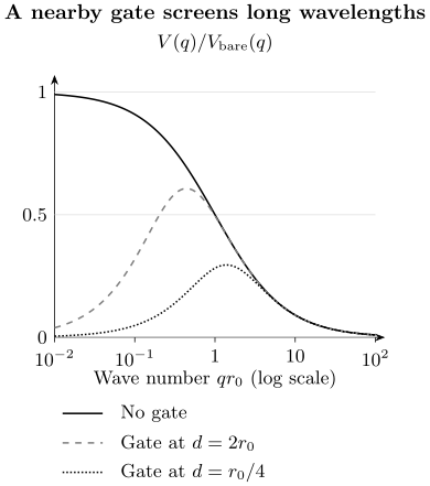
Calculated ratio $V(q)/V_{\mathrm{bare}}(q)$, where $V_{\mathrm{bare}}=e^2/(2\epsilon_0\kappa_{\mathrm{env}}q)$, for fixed sheet polarizability and dielectric environment. Small $q$ means long spatial wavelength. A grounded gate suppresses these long-wavelength interactions; a closer gate has the stronger effect. At large $qd$, the gated curves approach the ungated result. The model applies only while the sheet and dielectric continuum approximations remain valid.

This result is not universal to every stack: multiple gates, dielectric interfaces, anisotropy, finite thickness, or nonlocal polarization require the corresponding electrostatic response problem. Gate distance is part of the interaction Hamiltonian rather than only a device detail. Dynamic collective charge response belongs with Plasmons Preview, while carrier screening beyond this electrostatic model requires a polarization calculation.

Valleys and optical selection

A valley is a momentum-space label

A valley is a well-separated local extremum or low-energy pocket in momentum space. If two extrema at $\mathbf K_+$ and $\mathbf K_-$ are symmetry related, a label $\tau=\pm1$ can act as a low-energy pseudospin. The label is useful only when intervalley scattering is weak on the timescale of interest.

Time reversal relates opposite valleys. For a nonmagnetic spinful system,

$$\begin{aligned} E_{n,\tau,s}(\mathbf k) &= E_{n,-\tau,-s}(-\mathbf k), \\ \Omega_{n,\tau,s}(\mathbf k) &= -\Omega_{n,-\tau,-s}(-\mathbf k), \end{aligned}$$

where $\Omega$ is Berry curvature. If the momentum distributions also obey time reversal, their Berry-curvature contributions to the charge Hall response cancel, although the valleys can carry opposite transverse currents. Equal total carrier numbers alone are insufficient when different parts of the two valleys are populated. Exercise 4 makes this distinction explicit.

Not every two-dimensional band has a useful valley degree of freedom. The extrema must be distinct, long lived, and experimentally addressable. Edge disorder, short-range defects, phonons, exchange, and Coulomb scattering can transfer the large momentum needed to relax valley polarization.

Circular selection is a matrix-element statement

For light incident normal to a layer, define circular interband matrix elements

$$P_\pm(\mathbf k) = \left\langle u_{c\mathbf k} \middle| p_x\pm ip_y \middle| u_{v\mathbf k} \right\rangle .$$

A local circular dichroism measure is

$$\eta(\mathbf k) = \frac{|P_+|^2-|P_-|^2} {|P_+|^2+|P_-|^2}.$$

Broken inversion symmetry and orbital angular momentum can make $\eta$ have opposite signs in time-reversed valleys, as in idealized monolayer group-VI dichalcogenides (Xiao and collaborators, 2012). Spin–orbit coupling can further lock spin and valley labels near a band edge.

Circularly polarized photoluminescence is not by itself a direct population meter. Excitation detuning, exciton formation, exchange-driven depolarization, dark states, reabsorption, and polarization-dependent collection can all affect the measured helicity. A valley claim should combine selection rules with dynamics and at least one control that reverses the expected sign.

Excitons and optical gaps

Optical and quasiparticle gaps are different

An electron promoted across a semiconductor gap leaves a hole. Their attraction can bind an exciton with relative-coordinate equation

$$\left[ -\frac{\hbar^2}{2\mu}\nabla_{\mathbf r}^2 -V_{eh}(r) \right] \psi_\lambda(\mathbf r) = -E_{b,\lambda}\psi_\lambda(\mathbf r),$$

Here $\mu^{-1}=(m_e^\ast)^{-1}+(m_h^\ast)^{-1}$ is the reduced mass and $V_{eh}>0$ is the magnitude of the attraction. This relative-coordinate model assumes parabolic bands and an exciton spread over many unit cells. The neutral exciton transition is approximately

$$E_{X,\lambda} = E_g^{\mathrm{QP}} -E_{b,\lambda},$$

before phonon, exchange, disorder, and many-body shifts are included. Here $E_g^{\mathrm{QP}}$ is the electron–hole continuum threshold for the same band, spin and total-momentum channel as the exciton. For a direct band-edge exciton it can coincide with the fundamental quasiparticle gap; an indirect or optically dark lower channel need not. A Kohn–Sham eigenvalue difference is not generally this threshold.

For an ideal strictly two-dimensional $1/r$ interaction, the hydrogenic benchmark is

$$E_n = -\frac{\mathrm{Ry}^{\ast}} {(n-\tfrac12)^2}, \qquad n=1,2,\ldots,$$

with

$$\mathrm{Ry}^{\ast} = \frac{\mu e^4} {2(4\pi\epsilon_0\kappa_{\mathrm{env}})^2\hbar^2}.$$

The ground-state binding is $4\mathrm{Ry}^{\ast}$, four times the three-dimensional hydrogenic benchmark with the same $\mu$ and dielectric constant. Real monolayers are generally nonhydrogenic because the interaction crosses between logarithmic and Coulombic regimes, bands are not perfectly parabolic, and screening is frequency and environment dependent.

An optical peak may arise from a bright or dark exciton, a charged complex, an interlayer pair, a phonon sideband or a localized state. Polarization, gate dependence, temperature and lifetime help distinguish them; matching an energy alone is insufficient. Transition-Metal Dichalcogenides develops these assignments.

A photoluminescence peak alone does not determine binding energy. The neutral resonance must be compared with a defensible continuum threshold or an explicitly justified excited-state model. Chernikov and collaborators (2014) resolved a WS₂ exciton series whose level spacings depart from the constant-dielectric hydrogen model.

Stacking and interlayer excitons

Stacking creates a new Hamiltonian

Weak interlayer adhesion allows sheets with different lattice constants and chemistry to be assembled without the strict lattice matching demanded by conventional epitaxy. The layers can retain recognizable bands while acquiring tunnelling, electrostatic coupling, strain, and proximity interactions.

Band alignment	Single-particle starting point
Type I	The conduction minimum and valence maximum favor the same layer.
Type II	The electron and hole edges favor different layers, allowing interlayer excitons.
Type III	A conduction edge lies below the other layer’s valence edge, allowing charge transfer and interband tunnelling.

These labels describe a single-particle starting point. Hybridization, quasiparticle self-energy, interface dipoles, doping, strain, and exciton binding can revise the effective alignment.

For an interlayer exciton with charge separation $d_{eh}$, the out-of-plane dipole is approximately

$$p_z \simeq e\,d_{eh}.$$

Its leading Stark shift is

$$\Delta E_X \simeq -p_zE_z,$$

with sign fixed by the dipole orientation. A measured Stark slope probes the dipole only after the local electric field and transition assignment have been established.

The assembly and interface physics are developed in van der Waals Heterostructures; Geim and Grigorieva (2013) describe the basic approach. Weak interlayer bonding does not eliminate bubbles, strain, contamination or contact doping. Twist and lattice mismatch can create a moiré superlattice, whose geometric period alone does not establish a flat band or an interacting phase.

Gate voltage, density and chemical potential

Gate voltage is not identical to carrier density

Consider a contacted sheet in electrochemical equilibrium with one gate, neglecting traps and leakage. All capacitances below are per unit area. Let $n$ be excess electron number per area and $Q=en$ the positive gate charge per area that balances the sheet’s charge $-en$, with $e>0$. A small gate-voltage change divides between electrostatic charging and raising the sheet chemical potential:

$$\delta V_g = \frac{\delta Q}{C_{\mathrm{geom}}} + \frac{\delta\mu}{e}.$$

The thermodynamic density response defines the quantum capacitance (Luryi, 1988)

$$C_Q = e^2\frac{\partial n}{\partial\mu}.$$

For an ideal series combination,

$$\frac{1}{C_{\mathrm{tot}}} = \frac{1}{C_{\mathrm{geom}}} + \frac{1}{C_Q}.$$

When $C_Q\gg C_{\mathrm{geom}}>0$, the chemical-potential contribution is small, giving $en\simeq C_{\mathrm{geom}}(V_g-V_0)$ after calibrating the offset $V_0$. When $C_Q$ is small, much of the voltage instead changes $\mu$. The series relation uses a thermodynamic response: interactions can even make $\partial\mu/\partial n$ negative, so the simple “smaller positive capacitance wins” rule requires both capacitances to be positive. A stable uniform charging state requires a positive total inverse capacitance.

Dual gates separate density and displacement

With top and bottom gates, assume the chemical-potential voltage changes are negligible, as in the large-positive-$C_Q$ limit, and calibrate the voltage offsets. Then one convention is

$$\begin{aligned} en &= C_t(V_t-V_{t0}) + C_b(V_b-V_{b0}), \\ D &= \frac{1}{2} \left[ C_t(V_t-V_{t0}) -C_b(V_b-V_{b0}) \right]. \end{aligned}$$

Here $D$ has units of surface charge density; some authors divide by $\epsilon_0$ or reverse a sign. The convention must be stated. Independent density and displacement control is especially valuable in bilayers and heterostructures, where a transverse field can shift layer polarization or band alignment.

To change density without changing $D$, vary voltages so $C_t\delta V_t=C_b\delta V_b$. To change $D$ at fixed density, use $C_t\delta V_t=-C_b\delta V_b$. These relations follow directly by adding and subtracting the two gate-charge contributions. Near an incompressible gap, or with substantial trapped charge, solve the full electrostatics rather than treating this linear map as exact.

Exercises

Exercise 1: flexural fluctuation power counting

For a tensionless harmonic membrane, use $\langle|h_{\mathbf q}|^2\rangle\propto q^{-4}$ to determine how $\langle h^2\rangle$ depends on linear system size $L$ in two dimensions. What changes when finite tension dominates?

Solution

In two dimensions,

$$\left\langle h^2\right\rangle \propto \int_{2\pi/L}^{\Lambda} d^2q\,q^{-4} \propto \int_{2\pi/L}^{\Lambda} dq\,q^{-3}.$$

The infrared contribution scales as $L^2$ in the tensionless harmonic theory. If tension dominates, the denominator becomes $\sigma q^2$, so

$$\left\langle h^2\right\rangle_\sigma \propto \int dq\,q^{-1} \sim \ln L.$$

Real crystalline membranes require anharmonic coupling between bending and in-plane strain, which renormalizes this naive harmonic scaling.

Exercise 2: screening asymptotes

Explain from $V(q)\propto[q(1+r_0q)]^{-1}$ why the interaction approaches $1/r$ at $r\gg r_0$ and a logarithm at $r\ll r_0$.

Solution

Large real-space distance samples small $q$, where $1+r_0q\simeq1$. Thus $V(q)\propto1/q$, whose two-dimensional Fourier transform is proportional to $1/r$.

Short distance samples $q\gg r_0^{-1}$, where

$$V(q) \propto \frac{1}{r_0q^2}.$$

The two-dimensional Fourier transform of $1/q^2$ is logarithmic. The crossover is smooth, and the continuum model ceases to be reliable once $r$ approaches the lattice scale.

Exercise 3: ideal two-dimensional exciton

Compare the ideal two-dimensional and three-dimensional hydrogenic ground-state binding energies for the same reduced mass and dielectric constant. Give two reasons a monolayer semiconductor need not realize this ratio.

Solution

The three-dimensional ground state has $E_1^{3D}=-\mathrm{Ry}^{\ast}$. In two dimensions,

$$E_1^{2D} = -\frac{\mathrm{Ry}^{\ast}}{(1-\tfrac12)^2} = -4\mathrm{Ry}^{\ast}.$$

The ideal two-dimensional state is therefore four times more strongly bound. Real monolayers have nonlocal Rytova–Keldysh screening rather than a constant-dielectric $1/r$ interaction, and their bands can be nonparabolic or multivalley. Finite layer thickness, dielectric anisotropy, exchange, and dynamical screening provide additional corrections.

Exercise 4: when do valley Hall contributions cancel?

For two time-reversed valleys, assume $\Omega_-(-\mathbf k)=-\Omega_+(\mathbf k)$ and $f_-(-\mathbf k)=f_+(\mathbf k)$. Show that their intrinsic charge Hall conductivities cancel. Why would equal integrated carrier numbers alone be insufficient?

Solution

For one resolved band and valley, the intrinsic contribution is

$$\sigma_{xy}^{(\tau)}=-\frac{e^2}{\hbar} \int_\tau\frac{d^2k}{(2\pi)^2} f_\tau(\mathbf k)\Omega_\tau(\mathbf k).$$

Change variable $\mathbf k\mapsto-\mathbf k$ in the minus valley. The assumed distributions are identical under that change and the curvatures have opposite signs, so $\sigma_{xy}^{(-)}=-\sigma_{xy}^{(+)}$. The difference of valley contributions can remain nonzero.

Equal carrier numbers constrain only $\int f$, whereas the Hall response contains $\int f\Omega$. For example, one valley could populate states of curvature magnitude $\Omega_0$ and the other states of magnitude $2\Omega_0$, with equal numbers in each. Their opposite signs would not cancel their unequal weights. Such a distribution is not time-reversal invariant, despite equal valley populations. Spin partners must also be paired when spin is resolved.

Exercise 5: quantum-capacitance limit

Assume $C_Q,C_{\mathrm{geom}}>0$. Show that $C_{\mathrm{tot}}\simeq C_Q$ when $C_Q\ll C_{\mathrm{geom}}$ and $C_{\mathrm{tot}}\simeq C_{\mathrm{geom}}$ in the opposite limit. What does each regime measure?

Solution

From

$$C_{\mathrm{tot}} = \frac{C_{\mathrm{geom}}C_Q} {C_{\mathrm{geom}}+C_Q},$$

the smaller series capacitance controls the result. If $C_Q\ll C_{\mathrm{geom}}$, then $C_{\mathrm{tot}}\simeq C_Q$, making the measurement sensitive to thermodynamic density of states and compressibility. If $C_Q\gg C_{\mathrm{geom}}$, then $C_{\mathrm{tot}}\simeq C_{\mathrm{geom}}$, and ordinary electrostatics controls the gate conversion. Trap and stray capacitances must still be separated experimentally.

Exercise 6: interlayer-exciton Stark slope

An interlayer exciton has electron–hole separation $d_{eh}=0.7\,\mathrm{nm}$. Estimate the magnitude of its linear energy shift per electric field of $0.1\,\mathrm{V\,nm^{-1}}$.

Solution

Using $|\Delta E|=ed_{eh}|E_z|$,

$$\begin{aligned} d_{eh}|E_z| &= (0.7\,\mathrm{nm}) (0.1\,\mathrm{V\,nm^{-1}}) \\ &= 0.07\,\mathrm V, \\[3pt] |\Delta E| &= 0.07\,\mathrm{eV}. \end{aligned}$$

Thus the ideal dipole estimate is $70\,\mathrm{meV}$. The measured slope can differ because the electron and hole wave functions are not point charges, dielectric screening and hybridization change with field, and the local field may differ from the externally quoted displacement field.

References

• A. Chernikov et al., “Exciton Binding Energy and Nonhydrogenic Rydberg Series in Monolayer WS₂,” Physical Review Letters 113, 076802 (2014), doi:10.1103/PhysRevLett.113.076802.
• P. Cudazzo, I. V. Tokatly, and A. Rubio, “Dielectric Screening in Two-Dimensional Insulators: Implications for Excitonic and Impurity States in Graphane,” Physical Review B 84, 085406 (2011), doi:10.1103/PhysRevB.84.085406.
• A. K. Geim and I. V. Grigorieva, “Van der Waals Heterostructures,” Nature 499, 419–425 (2013), doi:10.1038/nature12385.
• L. H. Ho, A. P. Micolich, A. R. Hamilton, and O. P. Sushkov, “Ground-Plane Screening of Coulomb Interactions in Two-Dimensional Systems: How Effectively Can One Two-Dimensional System Screen Interactions in Another?”, Physical Review B 80, 155412 (2009), doi:10.1103/PhysRevB.80.155412.
• S. Luryi, “Quantum Capacitance Devices,” Applied Physics Letters 52, 501–503 (1988), doi:10.1063/1.99649.
• K. F. Mak, C. Lee, J. Hone, J. Shan, and T. F. Heinz, “Atomically Thin MoS₂: A New Direct-Gap Semiconductor,” Physical Review Letters 105, 136805 (2010), doi:10.1103/PhysRevLett.105.136805.
• J. C. Meyer et al., “The Structure of Suspended Graphene Sheets,” Nature 446, 60–63 (2007), doi:10.1038/nature05545.
• D. R. Nelson and L. Peliti, “Fluctuations in Membranes with Crystalline and Hexatic Order,” Journal de Physique 48, 1085–1092 (1987), doi:10.1051/jphys:019870048070108500.
• D. Xiao, G.-B. Liu, W. Feng, X. Xu, and W. Yao, “Coupled Spin and Valley Physics in Monolayers of MoS₂ and Other Group-VI Dichalcogenides,” Physical Review Letters 108, 196802 (2012), doi:10.1103/PhysRevLett.108.196802.