Engineered Heterostructures

An engineered heterostructure is a composite quantum system whose interface is designed to transfer, combine, or reshape selected properties of its constituents. A semiconductor may acquire pairing from a superconductor; a topological surface may acquire an exchange gap from a magnet; two insulating oxides may produce a conducting interface; or a cavity mode may hybridize with a material excitation. The useful object is not simply material A placed beside material B. It is the coupled system A–interface–B, including strain, electrostatics, disorder, electromagnetic boundary conditions, and contacts.

The same coupling that transfers a useful interaction can also transfer disorder and dissipation. We will compare four examples through their simplest models: induced superconductivity, exchange-gapped surface states, polar oxide interfaces and coupled light–matter modes.

Required background. van der Waals Heterostructures supplies stacking, hybridization and interface control. Proximity and Andreev Physics supplies induced superconducting correlations and interface diagnostics. Topological Insulators supplies the distinction between bulk topology and conducting boundary signals. Two-Dimensional Electron Gases supplies the confinement, density and disorder scales of populated interfaces.

How coupling changes an electronic state

An electron can leave one layer, propagate in the other, and return. The effective Hamiltonian of the first layer must include this process. Its amplitude depends on energy, so the interface cannot generally be represented by one constant induced potential.

A transferred property is a frequency-dependent response

For two ordinary electron sectors of a quadratic single-particle Hamiltonian, use the retarded energy argument $z=E+i0^+$, with $E$ measured relative to the common chemical potential $\mu$. Block inversion gives

$$\begin{aligned} G_A^{-1}(z,\mathbf k) ={}&z+\mu-H_A(\mathbf k) -\Sigma_A(z,\mathbf k), \\ \Sigma_A(z,\mathbf k) ={}&T(\mathbf k) G_B^{(0)}(z,\mathbf k) T^\dagger(\mathbf k), \\ G_B^{(0)}(z,\mathbf k) ={}&[z+\mu-H_B(\mathbf k)]^{-1}. \end{aligned}$$

For a superconducting Nambu description, instead form the specified BdG Hamiltonian with the chemical potential already included in its particle and hole blocks, and use the resolvent $[zI-H_{\mathrm{BdG}}]^{-1}$; there is no additional scalar $+\mu I$. The same block-inversion identity then applies with the Nambu tunneling matrix.

The interface self-energy is $\Sigma_A$, not the isolated-parent resolvent $G_B^{(0)}$. Its Hermitian part shifts levels, changes velocities, opens avoided crossings, and can induce exchange or, in the Nambu extension, pairing. Its retarded anti-Hermitian part describes escape into a continuum or a specified broadened parent; an isolated finite Hermitian sector B instead has discrete hybridization poles. Energy dependence redistributes spectral weight and renormalizes parameters in A. An angular frequency would enter as $\hbar\omega$, not as an energy-valued $\omega$.

This identity by itself does not supply interfacial many-body self-energies, electrostatic readjustment, or feedback that suppresses the parent order; those require further model inputs. It isolates the hybridization-mediated part of the interface response.

This compact expression explains why “stronger coupling” is not an unconditional improvement. Increasing $T$ can enlarge the desired induced scale while also:

• transferring disorder, quasiparticle poisoning, or dissipation;
• reducing the quasiparticle weight that remains in the controllable subsystem;
• producing charge transfer and band bending that move the chemical potential;
• straining or chemically reconstructing the interface;
• degrading the parent order through inverse proximity.

The full derivation and the distinction between hybridization, electrostatics, and proximity are developed in van der Waals Heterostructures.

An induced gap and its subgap spectral weight answer different questions: the gap measures an energy scale, while unwanted states inside it can still carry current or cause relaxation. Likewise, a mode splitting must be compared with the decay rates of both modes.

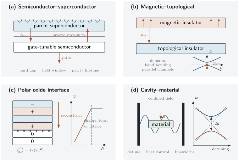
Four ways an interface changes a system: superconducting pairing, magnetic exchange, charge redistribution and light–matter hybridization. The sketches illustrate mechanisms, not measured phase diagrams.

Semiconductor–Superconductor Devices

The useful compromise

A low-density semiconductor provides electrostatic control, strong spin–orbit coupling, and a large effective $g$ factor; a conventional superconductor provides a condensate and a hard excitation gap. Chang and collaborators showed with epitaxial InAs–Al hybrids that atomic-scale interface control can greatly suppress the soft subgap continuum that limited earlier devices. Planar two-dimensional electron gases, selective-area networks, nanowires, and Josephson junctions now realize complementary geometries.

The design objective is not to maximize the induced gap alone. In a simple low-energy proximity model, stronger semiconductor–superconductor coupling increases the induced pairing toward the parent gap while moving spectral weight into the metal. The same process can reduce the semiconductor’s effective Zeeman and spin–orbit scales. A thin parent film can raise the critical field for a favorable orientation, yet orbital depairing, vortices, and disorder still constrain the usable field window.

This parameter renormalization is developed by Stanescu and Das Sarma. The induced-gap self-energy and scattering diagnostics are derived in Proximity and Andreev Physics; use parameters of the coupled device, rather than the bare semiconductor, in an effective low-energy model.

Topological operation is a stricter claim

In the ideal uniform single-subband Rashba-wire model of Lutchyn, Sau and Das Sarma and Oreg, Refael and von Oppen, the bulk transition is located by

$$V_Z^2 = \mu^2+\Delta_{\mathrm{ind}}^2,$$

with the topological side at larger $V_Z$ while a reopened excitation gap survives. Here $V_Z$ is the effective Zeeman energy, $\mu$ the chemical potential relative to the subband crossing, and $\Delta_{\mathrm{ind}}$ the effective pairing amplitude. The criterion assumes nonzero spin–orbit coupling and an appropriate field orientation. It locates a transition in that model. Multiband occupation, smooth confinement, disorder, orbital coupling, parent-gap collapse, and interactions can all produce low-energy states outside its assumptions.

A local zero-bias peak is therefore insufficient. Stronger evidence includes a resolved bulk gap closing and reopening, correlated end response, length dependence, nonlocal conductance, calibrated temperature and lead transmission, parity-sensitive measurements, and eventually fusion or braid-order protocols. The topological-superconductor guide explains the invariant and why the measurement must distinguish a protected mode from an ordinary low-energy Andreev state.

Magnetic–Topological Interfaces

Which component of exchange opens the gap?

The low-energy surface of an ideal three-dimensional topological insulator can be modeled as

$$H_{\mathrm{surf}} = \hbar v_F \left( k_x\sigma_y-k_y\sigma_x \right) + \mathbf m\cdot\boldsymbol{\sigma} + V_0.$$

An out-of-plane exchange component $m_z\sigma_z$ anticommutes with the kinetic term and opens a Dirac mass gap $2\lvert m_z\rvert$. Uniform in-plane components mainly shift the Dirac point in momentum in this minimal model. Real interfaces also add warping, potential disorder, hybridization, band bending, and symmetry-lowering terms, so magnetization by itself does not determine the spectrum.

The design must satisfy four conditions at once:

1. the magnetic layer has the required orientation and domain structure;
2. exchange reaches the topological electronic state rather than only a remote band;
3. the chemical potential lies in a global mobility gap;
4. side surfaces, opposite surfaces, domains, and parallel bulk channels do not short the response.

For the displayed Hamiltonian, fixed $(k_x,k_y)$ orientation, and the volume Hall convention, the occupied lower cone contributes

$$\sigma_{xy}^{\mathrm{cone}} = -\frac{e^2}{2h} \operatorname{sgn}(m_z),$$

when the chemical potential lies in its mass gap. A physical surface also has an ultraviolet/background contribution fixed by its bulk and surface completion. It cannot be determined from this continuum cone alone. At fixed completion, reversing the mass from negative to positive changes this contribution by $-e^2/h$. A complete finite sample has an integer-consistent electromagnetic response after the other surfaces and channels are included; the half value is not a stand-alone two-dimensional lattice Chern number.

Connecting the exchange gap to transport

An anomalous Hall loop proves neither an exchange-gapped Dirac cone nor a quantum anomalous Hall state. Stray fields, magnetic impurities, ordinary multiband Berry curvature, and parallel conduction can produce superficially similar responses. Conversely, a spectroscopic gap at the Dirac energy can arise from hybridization, disorder, or matrix-element effects without long-range time-reversal breaking.

Interface-sensitive magnetometry can test whether exchange reaches the electronic surface state. Spectroscopy locates the electronic gap; gate dependence and longitudinal transport test whether other channels bypass it. Quantized Hall transport is a stronger condition than an anomalous Hall loop. The experiment of Chang and collaborators established the quantum anomalous Hall effect in a magnetically doped topological-insulator film; it does not imply that every magnetic interface produces it.

Oxide Interfaces

Polar discontinuity is a boundary condition, not a complete mechanism

Perovskite oxides bring charge, spin, orbital, and lattice degrees of freedom onto similar energy scales. The LaAlO$_3$/SrTiO$_3$ interface joins band insulators yet can conduct, as demonstrated by Ohtomo and Hwang, and become superconducting, as shown by Reyren and collaborators.

Along the (001) direction, ideal LaAlO$_3$ consists of alternating charged $(\mathrm{LaO})^+$ and $(\mathrm{AlO}_2)^-$ planes, whereas ideal SrTiO$_3$ has neutral $(\mathrm{SrO})^0$ and $(\mathrm{TiO}_2)^0$ planes. If uncompensated, the electric field in a polar film gives an electrostatic potential that grows approximately with its thickness:

$$\Delta V_N \simeq \frac{N\sigma_0 d} {\epsilon_0\epsilon_{\mathrm{LAO}}},$$

Here $N$ counts full polar repeats of length $d$, and $\sigma_0$ denotes the effective macroscopic polar charge producing the repeat-averaged field. For ideal alternating ionic planes $\pm\sigma_{\mathrm{ion}}$ separated by $d/2$, with zero external field on the nonpolar side, that average field is $\sigma_{\mathrm{ion}}/(2\epsilon_0\epsilon_{\mathrm{LAO}})$, so this convention uses $\sigma_0=\sigma_{\mathrm{ion}}/2$. It does not identify $\sigma_0$ with the full charge of a single ionic plane. Once the energy cost becomes large enough, the system must reconstruct electronically, ionically, chemically, or structurally.

In the ideal electronic-reconstruction count, half an electron per in-plane unit cell reaches the $n$-type interface:

$$n_{2D}^{(0)} = \frac{1}{2a^2} \simeq 3.3\times10^{14}\ {\rm cm}^{-2}.$$

Here $a\simeq3.9\ {\rm \mathring A}$ is the in-plane lattice constant. This number is a formal compensation scale, not a prediction that every Hall measurement must return it. Localized charge, multiple bands, oxygen vacancies, cation intermixing, surface adsorbates, ferroelectric-like lattice polarization, and incomplete transfer all alter the mobile density.

The interface selects orbitals as well as charge

Confinement and broken cubic symmetry split the Ti $t_{2g}$ manifold. The more strongly confined $d_{xy}$-derived states can lie below the $d_{xz}$ and $d_{yz}$ states, while interactions and atomic spin–orbit coupling mix this simple orbital picture. Gate voltage then changes not only the number of carriers but also which subbands, orbitals, and spatial regions conduct.

This matters when interpreting coexistence. Superconducting transport below a few hundred millikelvin and magnetic or hysteretic signals can occur in the same nominal device without proving a homogeneous microscopic phase. Spatial inhomogeneity, phase separation, localized moments near defects, and different orbital populations can make distinct probes weight different regions.

The termination and oxygen environment help determine which compensating mechanism occurs. A Hall density probes mobile charge through a transport model; it need not equal the total compensating charge inferred from electrostatics.

Cavity–Material Hybrids

An anticrossing is the beginning of the analysis

A material resonance of frequency $\omega_m$ coupled to a cavity mode $\omega_c$ has the elementary non-Hermitian mode matrix

$$\mathcal M = \begin{pmatrix} \omega_c-i\kappa/2 & g \\ g & \omega_m-i\gamma/2 \end{pmatrix},$$

Here $g$, $\kappa$ and $\gamma$ are angular-frequency rates. The positive quantities $\kappa$ and $\gamma$ are energy or occupation decay rates, so the amplitudes decay at half those rates. For an isolated Lorentzian they are also full widths at half maximum. In the lossless resonant limit, the normal modes split by $2g$. Away from resonance,

$$\omega_\pm = \frac{\omega_c+\omega_m}{2} \pm \sqrt{ g^2+\frac{(\omega_c-\omega_m)^2}{4} }.$$

Angle-, field-, gate-, or length-dependent tracking of both branches distinguishes hybridization from two unrelated peaks. The cooperativity $C=4g^2/(\kappa\gamma)$ is a useful dimensionless measure, but $C>1$ and a visually resolved doublet are not identical criteria; linewidth conventions and experimental geometry must be stated.

The semiconductor microcavity experiment of Weisbuch and collaborators is a classic example of coupled exciton–photon modes. Cyclotron transitions in high-mobility two-dimensional electron gases have reached the ultrastrong-coupling regime. When

$$\eta = \frac{g}{\omega_c} \gtrsim 0.1,$$

counter-rotating and diamagnetic terms can no longer be omitted casually. Gauge-consistent truncation is essential: deleting the quadratic light–matter term in one gauge while retaining its consequences in another can create spurious ground-state predictions.

Polariton formation is not automatically phase control

Two coupled linear oscillators already produce an avoided crossing. That observation establishes hybridized excitations under the model assumptions; it does not establish a new equilibrium ordered phase. Driven polariton populations also depend on pumping and loss.

For a proposed cavity-induced change of material properties, compare a detuned or field-node control, quantify heating, and measure the material response as well as the optical spectrum. Schlawin, Kennes and Sentef discuss these distinctions. As a concrete experimental example, Helmrich and collaborators reported a cavity-induced bound resonance emerging from bilayer graphene’s interband continuum. A bound excitation and a new many-body phase are different conclusions.

Proximity-Engineered Phases

Inherited amplitude, hybrid state, or new phase?

The word proximity covers physically different outcomes.

Outcome	Diagnostic meaning	Example
inherited response	A acquires a small order-parameter component or splitting tied to B	induced pair amplitude in a normal layer
hybridized excitation	eigenstates have appreciable weight in both subsystems	exciton–polariton or avoided band crossing
reconstructed interface	charge, orbital, or lattice structure changes near the boundary	oxide two-dimensional electron liquid
engineered phase	the coupled bulk has a gap and phase label not possessed by either parent	an appropriate topological superconducting phase

The distinction is operational. A hybridized spectrum can exist above any ordering temperature. An inherited anomalous signal can be local and nonuniform. A topological label requires a bulk or defect invariant under stated symmetries and a protecting gap, not merely the presence of ingredients associated with a proposal.

A useful design must retain the desired interaction and its operating conditions. For example, a field large enough to enter a model’s topological regime is useless if it has already destroyed the parent superconducting gap. Exercise 1 makes this competing-scale test explicit.

Exercises

1. Field window in an ideal hybrid wire

Assume an ideal single-subband model with $\mu=0.20\ {\rm meV}$, $\Delta_{\mathrm{ind}}=0.25\ {\rm meV}$, effective $g$ factor $g^\ast=15$, and

$$V_Z = \frac{1}{2}g^\ast\mu_B B, \qquad \mu_B=57.88\ {\rm \mu eV\,T^{-1}}.$$

Find the model transition field. If the parent gap collapses at $1.2\ {\rm T}$, is there an idealized field window above the transition?

Solution

The transition Zeeman energy is

$$\begin{aligned} V_Z^{(c)} &= \sqrt{ \mu^2+\Delta_{\mathrm{ind}}^2 } \\ &= \sqrt{ (0.20)^2+(0.25)^2 }\ {\rm meV} \\ &\simeq 0.320\ {\rm meV}. \end{aligned}$$

The Zeeman coefficient is

$$\begin{aligned} \frac{1}{2}g^\ast\mu_B &= \frac{15}{2} \left( 0.05788\ {\rm meV\,T^{-1}} \right) \\ &\simeq 0.434\ {\rm meV\,T^{-1}}. \end{aligned}$$

so

$$B_c \simeq \frac{0.320}{0.434}\ {\rm T} \simeq 0.74\ {\rm T}.$$

The ideal model leaves a nominal interval $0.74\ {\rm T}<B<1.2\ {\rm T}$. This arithmetic does not prove that the reopened gap is hard or topological: orbital depairing, multiple subbands, disorder, and field-dependent renormalization can close the useful window.

2. Which exchange direction gaps a Dirac surface?

For

$$H = \hbar v_F \left( k_x\sigma_y-k_y\sigma_x \right) + m_x\sigma_x+m_z\sigma_z,$$

find the spectrum and identify the effects of $m_x$ and $m_z$.

Solution

Collecting Pauli-matrix coefficients gives

$$H ={} \left( m_x-\hbar v_F k_y \right)\sigma_x + \hbar v_F k_x\sigma_y + m_z\sigma_z.$$

Therefore

$$\begin{aligned} \varepsilon^2(\mathbf k) ={}& \left( \hbar v_F k_x \right)^2 + \left( m_x-\hbar v_F k_y \right)^2 +m_z^2, \\ E_\pm(\mathbf k) ={}& \pm\varepsilon(\mathbf k). \end{aligned}$$

The in-plane term shifts the cone to $k_y=m_x/(\hbar v_F)$ in this isotropic model. The perpendicular term opens a gap $2\lvert m_z\rvert$. Warping and lower interface symmetry can modify this clean separation.

3. Formal charge at a polar oxide interface

Using $a=3.905\ {\rm \mathring A}$, compute the sheet density corresponding to half an electron per in-plane unit cell. Compare it with a measured mobile density of $4.0\times10^{13}\ {\rm cm}^{-2}$.

Solution

The formal compensation density is

$$n_{2D}^{(0)} = \frac{1}{2a^2}.$$

Since $a=3.905\times10^{-8}\ {\rm cm}$,

$$\begin{aligned} n_{2D}^{(0)} &= \frac{1}{ 2(3.905\times10^{-8}\ {\rm cm})^2 } \\ &\simeq 3.28\times10^{14}\ {\rm cm}^{-2}. \end{aligned}$$

The measured mobile fraction is

$$\frac{ 4.0\times10^{13} }{ 3.28\times10^{14} } \simeq 0.12.$$

The mismatch does not refute polar compensation. Much of the compensating charge may be localized or distributed among poorly conducting states, while defects and multiband Hall factors can also alter the inferred mobile density.

4. Cavity anticrossing and composition

For the lossless two-mode model at detuning $\delta=\omega_c-\omega_m$, show that the splitting is $\sqrt{\delta^2+4g^2}$. At resonance, what fraction of each normalized eigenmode lies in the cavity and material sectors?

Solution

Subtracting the mean frequency $(\omega_c+\omega_m)/2$ leaves

$$\begin{pmatrix} \delta/2 & g \\ g & -\delta/2 \end{pmatrix}.$$

Its eigenvalues are

$$\lambda_\pm = \pm \sqrt{ g^2+\frac{\delta^2}{4} },$$

so the branch separation is

$$\omega_+-\omega_- = \sqrt{ \delta^2+4g^2 }.$$

At $\delta=0$, the normalized eigenvectors are proportional to $(1,1)$ and $(1,-1)$. Each branch has cavity weight $1/2$ and material weight $1/2$ in this ideal lossless model.

5. Coupling versus loss

Two cavity–material devices have parameters

$$\begin{array}{c|ccc} & g & \kappa & \gamma \\ \hline \mathrm{A} & 4 & 8 & 2 \\ \mathrm{B} & 6 & 18 & 1 \end{array}$$

in the same frequency units. Compute the cooperativity of each. Explain why the larger $g$ does not by itself identify the cleaner hybrid.

Solution

Using $C=4g^2/(\kappa\gamma)$,

$$C_{\mathrm A} = \frac{4(4)^2}{(8)(2)} = 4,$$

whereas

$$C_{\mathrm B} = \frac{4(6)^2}{(18)(1)} = 8.$$

Device B has the larger cooperativity. To compare spectral scales, diagonalize the lossy matrix at resonance:

$$\omega_\pm=\omega_0-i\frac{\kappa+\gamma}{4} \pm\sqrt{g^2-\frac{(\kappa-\gamma)^2}{16}}.$$

For A, the real pole separation is $7.42$ and each pole has full linewidth $5$. For B, the separation is $8.47$ but the linewidth is $9.5$. Thus B’s larger cooperativity does not mean better separated resonances. Distinct real parts require $g>\lvert\kappa-\gamma\rvert/4$, but resolving two peaks also depends on which mode is driven and detected; pole separation alone does not determine the measured line shape.

6. Interpreting a magnetic interface

A ferromagnet is deposited on a topological-insulator film. The device shows a hysteretic Hall resistance and a gap-like depression in photoemission, both disappearing near the ferromagnet’s Curie temperature. Longitudinal resistance remains finite, and the chemical potential is not independently located. Classify what is established and list four measurements needed for a quantum anomalous Hall claim.

Solution

The observations support magnetic coupling correlated with the ferromagnet and a temperature-dependent electronic reconstruction. They are compatible with an exchange-gapped topological surface, but they do not establish a global Chern-insulating phase.

Four stronger checks are:

1. gate or spectroscopic determination that the chemical potential lies inside a global mobility gap;
2. accurately quantized Hall resistance together with longitudinal resistance approaching zero;
3. interface-sensitive magnetic characterization and domain control;
4. nonlocal transport or spatial imaging consistent with chiral edge conduction.

Structural controls, a nonmagnetic reference, thickness dependence, and tests for parallel bulk channels would strengthen the causal assignment further.

Further connections

2D Magnets and Ferroelectrics explains layer-resolved magnetic order. Two-Dimensional Electron Gases develops subband occupation and transport, while Cavity QED treats driven, dissipative light–matter dynamics. Quantum Materials by Design connects the desired response to material selection and synthesis.

References

• C.-Z. Chang et al., “Experimental Observation of the Quantum Anomalous Hall Effect in a Magnetic Topological Insulator,” Science 340, 167–170 (2013), doi:10.1126/science.1234414.
• W. Chang et al., “Hard Gap in Epitaxial Semiconductor–Superconductor Nanowires,” Nature Nanotechnology 10, 232–236 (2015), doi:10.1038/nnano.2014.306.
• F. Helmrich et al., “Cavity-Driven Attractive Interactions in Quantum Materials,” Nature 654, 361–368 (2026), doi:10.1038/s41586-026-10609-1.
• R. M. Lutchyn, J. D. Sau, and S. Das Sarma, “Majorana Fermions and a Topological Phase Transition in Semiconductor–Superconductor Heterostructures,” Physical Review Letters 105, 077001 (2010), doi:10.1103/PhysRevLett.105.077001.
• A. Ohtomo and H. Y. Hwang, “A High-Mobility Electron Gas at the LaAlO$_3$/SrTiO$_3$ Heterointerface,” Nature 427, 423–426 (2004), doi:10.1038/nature02308.
• Y. Oreg, G. Refael, and F. von Oppen, “Helical Liquids and Majorana Bound States in Quantum Wires,” Physical Review Letters 105, 177002 (2010), doi:10.1103/PhysRevLett.105.177002.
• X.-L. Qi, T. L. Hughes, and S.-C. Zhang, “Topological Field Theory of Time-Reversal Invariant Insulators,” Physical Review B 78, 195424 (2008), doi:10.1103/PhysRevB.78.195424.
• N. Reyren et al., “Superconducting Interfaces between Insulating Oxides,” Science 317, 1196–1199 (2007), doi:10.1126/science.1146006.
• F. Schlawin, D. M. Kennes, and M. A. Sentef, “Cavity Quantum Materials,” Applied Physics Reviews 9, 011312 (2022), doi:10.1063/5.0083825.
• T. D. Stanescu and S. Das Sarma, “Proximity-Induced Low-Energy Renormalization in Hybrid Semiconductor–Superconductor Majorana Structures,” Physical Review B 96, 014510 (2017), doi:10.1103/PhysRevB.96.014510, arXiv:1702.03976.
• C. Weisbuch et al., “Observation of the Coupled Exciton–Photon Mode Splitting in a Semiconductor Quantum Microcavity,” Physical Review Letters 69, 3314–3317 (1992), doi:10.1103/PhysRevLett.69.3314.