Quantum Materials by Design

Quantum-materials design starts with a desired response and asks which structures and interactions could produce it. A useful target might be a Hall plateau over a stated temperature range, a long spin lifetime or an electrically switchable polarization. Composition, crystal symmetry, interfaces and defects all affect whether the response survives in a real sample.

The challenge is to connect three questions: does a model predict the response, can the material be made, and does the measurement identify that response? We will use competing-phase energies, symmetry constraints and simple uncertainty calculations to see why these questions require different answers.

Required background. From Models to Measured Observables supplies the separation of microscopic inputs, effective models and measured observables. Topology in Quantum Matter supplies the constraints and diagnostics behind a topological target. Low-Dimensional Quantum Matter supplies dimensional crossover and fluctuation limits. Hubbard Physics in Materials supplies the active-subspace, screening and parameter-validation requirements for a correlated-material model.

Choosing a response and comparing candidates

Specify the operating temperature, field, frequency and sample geometry along with the target observable. A material with the largest calculated gap may be difficult to synthesize; an easier material may lose the desired response after contacts or a substrate are added. These are competing objectives, not one universal quality score.

Let $f_i(x)$ be an objective for candidate $x$, with its direction chosen so larger is better. For example, the objectives might be a larger useful gap, a more reliable synthesis route and lower cost (represented by minus the cost).

For objectives to be maximized, candidate $x$ Pareto-dominates $y$ when

$$\begin{aligned} f_i(x)&\ge f_i(y) \quad\text{for every }i, \\ f_j(x)&>f_j(y) \quad\text{for at least one }j. \end{aligned}$$

Candidates not dominated by any other form a Pareto front. Choosing among them requires an explicit scientific or engineering preference. Hiding those preferences inside a weighted score can make a ranking look objective while merely encoding unreported weights.

A failed synthesis can reveal a missing competing phase or inaccessible reaction path; a missing electrical response can reveal an incorrect Fermi level or excessive disorder. Those results help refine the model and select the next experiment. Computational Quantum Matter introduces the electronic-structure methods used in these comparisons.

Stability Is a Hierarchy

Formation energy is only the first comparison

For one formula unit of a compound $M$ containing $n_a$ atoms of element $a$, a zero-temperature formation energy relative to chosen elemental reference states is

$$\Delta H_f(M) = E_{\mathrm{tot}}(M) - \sum_a n_a\mu_a^{\mathrm{elem}}.$$

A negative formation energy means that $M$ is favored over those elemental references within the calculation. It does not establish stability against decomposition into other compounds.

For convex-hull comparisons, switch to per-atom energies $\bar E_j=E_{\mathrm{tot}}(j)/N_j$ and atomic-fraction vectors $\mathbf x_j$, where $N_j=\sum_a n_{j,a}$ and $x_{j,a}=n_{j,a}/N_j$. Thus $\sum_a x_{j,a}=1$, and $\lambda_j$ below is the fraction of atoms assigned to phase $j$, not the number of its formula units. Include the candidate itself among the phases in the minimization. At fixed overall composition $\mathbf x_M$, the nonnegative energy above this hull per atom is

$$\begin{aligned} E_{\mathrm{hull}}(M) ={}& \bar E(M)-\bar E_{\mathrm{mix}}^{\min}, \\ \bar E_{\mathrm{mix}}^{\min} ={}& \min_{\{\lambda_j\}} \sum_j\lambda_j\bar E_j, \end{aligned}$$

subject to

$$\begin{aligned} \lambda_j&\ge0, & \sum_j\lambda_j&=1, \\ \sum_j\lambda_j\mathbf x_j &= \mathbf x_M. \end{aligned}$$

$E_{\mathrm{hull}}=0$ means stable against the included competing phases at the stated computational level. A positive value means thermodynamically unfavorable relative to some included decomposition mixture. It does not alone establish a metastable local minimum: that requires local stability and kinetic trapping, not merely a positive scalar energy difference. The per-atom excess-energy comparison used by Sun and collaborators measures one part of this thermodynamic and kinetic distinction. The hull can change when a missing polymorph is found, magnetic order is altered, numerical settings change, or a more accurate energy model is used.

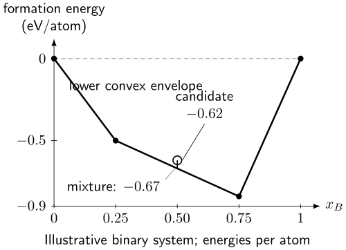
A negative formation energy does not guarantee stability. In this illustrative binary system, equal atom fractions of the phases at $x_B=0.25$ and $0.75$ produce $x_B=0.50$ at $-0.67$ eV/atom. The candidate at $-0.62$ eV/atom lies 50 meV/atom above that mixture. The lower convex envelope compares all included phases, not just the elements.

Temperature, pressure, and reservoirs matter

At finite temperature and in open chemical environments, a relevant potential may contain

$$\Phi ={} E_{\mathrm{el}} +F_{\mathrm{vib}}(T) +\Delta F_{\mathrm{el}}(T) +pV -TS_{\mathrm{conf}} -\sum_a \mu_aN_a.$$

Include the reservoir term only for species exchanged with the environment; closed-composition comparisons instead fix their amounts. All terms use the same extensive normalization, $E_{\mathrm{el}}=F_{\mathrm{el}}(0)$, and $\Delta F_{\mathrm{el}}(T)=F_{\mathrm{el}}(T)-F_{\mathrm{el}}(0)$ is only the electronic thermal correction; adding the full electronic free energy again would double count its zero-temperature part. Vibrational and configurational entropy can reorder close polymorphs. Gas partial pressures and chemical potentials matter for oxides, hydrides, chalcogenides, and growth under flux. Surfaces and interfaces alter the balance in thin films and nanoparticles. A zero-kelvin bulk hull is therefore one layer of evidence, not the whole synthesis problem.

Stability does not imply synthesizability

Four further questions are distinct:

• Dynamical stability: does the harmonic force-constant matrix have nonnegative squared frequencies, apart from allowed zero modes, at the tested structure? Finite-temperature anharmonic stabilization requires more than this zero-temperature test.
• Mechanical stability: does the elastic tensor satisfy the appropriate stability conditions?
• Kinetic accessibility: can available precursors reach the phase before becoming trapped in intermediates or losing volatile components?
• Persistence: does the product survive cooling, air exposure, cycling, and measurement?

Conversely, many useful materials are metastable. Epitaxy, pressure quenching, topotactic reactions, rapid cooling, ion exchange, and nanoscale confinement can select states above the bulk equilibrium hull. The correct design question is not “is $E_{\mathrm{hull}}$ below one universal cutoff?” It is “what thermodynamic and kinetic evidence supports this synthesis route for this material class?”

Symmetry and Topology as Design Principles

Work backward from the protected response

Symmetry can turn an unconstrained search into a structured one. Start with:

1. the relevant space or magnetic space group;
2. Wyckoff positions and site symmetries;
3. active orbital characters and electron filling;
4. spin–orbit, exchange, crystal-field, and hybridization scales;
5. the symmetry preserved by the bulk, surface, substrate, strain, and magnetic state;
6. the observable expected from the proposed topology.

For an isolated group of weakly interacting bands, let $\mathbf n$ collect the multiplicities of irreducible representations at high-symmetry momenta. Compatibility requires

$$\mathcal C\mathbf n = \mathbf0.$$

Atomic band representations generate vectors $\mathbf b_\alpha$. If

$$\mathbf n = \sum_\alpha q_\alpha\mathbf b_\alpha, \qquad q_\alpha\in\mathbb Z_{\ge0},$$

then the symmetry data are compatible with an atomic limit under the stated assumptions. Failure of such a nonnegative decomposition can diagnose an obstruction. Symmetry indicators package related quotient information and enable large-scale screening.

Symmetry of Bloch States explains the representation labels and compatibility relations. Bradlyn and collaborators and Po, Vishwanath and Watanabe develop these band-screening approaches. Compatibility with atomic symmetry labels alone does not prove that the full Bloch eigenstates have a localized atomic description.

The inference has limits:

• a nonzero indicator can certify topology only within its symmetry, gap, filling, and band-theory assumptions;
• a zero indicator does not exclude topology invisible to that indicator;
• incompatible labels may describe a symmetry-enforced semimetal rather than an insulator;
• DFT can misorder bands, underestimate gaps, or choose the wrong magnetic state;
• strong interactions can invalidate a one-electron classification or replace it with a many-body problem.

A topological candidate is not yet a useful material

After a band diagnosis, one must still determine:

• whether the relevant spectral or mobility gap survives the operating temperature and disorder; spectroscopic resolution is a separate constraint;
• whether the chemical potential can be placed in the relevant gap;
• whether surface or edge states survive the actual termination and reconstruction;
• whether trivial accumulation layers, bulk carriers, or magnetic domains mimic the signal;
• whether contacts and fabrication preserve the protecting symmetry;
• whether transport, spectroscopy, and thermodynamics support one consistent mechanism.

Symmetry and topology are powerful filters because they state necessary structure. They do not remove chemistry, defects, or experimental identification from the problem.

Correlation and Dimensionality as Design Knobs

Use a scale vector, not a single ratio

A first pass through a correlated candidate can be organized by

$$\begin{aligned} \boldsymbol{\eta}_{\mathrm{el}} &= \left( \frac{U}{W}, \frac{J_{\mathrm H}}{W}, \frac{\lambda_{\mathrm{SO}}}{W}, \frac{t_\perp}{t_\parallel} \right), \\ \boldsymbol{\eta}_{\mathrm{env}} &= \left( \frac{k_{\mathrm B}T}{W}, \frac{\Gamma_{\mathrm{dis}}}{W}, \frac{\hbar\omega_{\mathrm{ph}}}{W} \right). \end{aligned}$$

$\boldsymbol{\eta}_{\mathrm{el}}$ collects electronic design ratios and $\boldsymbol{\eta}_{\mathrm{env}}$ collects operating and environmental ratios. $U$ and $J_{\mathrm H}$ summarize screened interactions in a stated active basis; $W$ is the relevant bandwidth; $\lambda_{\mathrm{SO}}$ measures spin–orbit coupling; $t_\perp/t_\parallel$ measures dimensional crossover; and $\Gamma_{\mathrm{dis}}$ and $\omega_{\mathrm{ph}}$ represent disorder and lattice scales. None is a universal material constant independent of orbital choice, screening environment, structure, and probe window.

Layered chemistry, epitaxial strain, pressure, gating, dielectric screening, moiré periodicity, and interfacial hybridization can move several entries of $\boldsymbol{\eta}$. This makes them genuine design knobs, but not independent ones. Reducing $W$ raises $U/W$, yet can also:

• increase sensitivity to inhomogeneity and localization;
• strengthen electron–phonon competition;
• reduce phase stiffness and coherence scales;
• make neglected longer-range interactions important;
• amplify uncertainty in small hopping parameters.

A narrow band is therefore an opportunity for competing orders, not a phase prescription. Flat Bands develops the additional roles of isolation and quantum geometry.

Dimensional reduction changes fluctuations and fabrication

Lower dimension can enhance interaction effects and increase electrostatic tunability. It can also strengthen thermal fluctuations, environmental screening changes, substrate coupling, edge effects, and sample-to-sample disorder. Low-Dimensional Quantum Matter develops the density-of-states and fluctuation analysis.

For design, dimensionality should be reported through measured or computed crossover scales: occupied subband spacing, interlayer hopping, coherence lengths, screening length, thickness dependence, and the temperature at which neighboring layers lock together. Calling a material “two-dimensional” from morphology alone is not enough.

Correlated calculations need wider uncertainty budgets

When $U/W$ or multiorbital competition is large, semilocal DFT screening may still generate structures and broad trends, but its property ranking can be unreliable. A stronger workflow records the active orbitals, magnetic initial states, interaction parameters, double counting, solver, and sensitivity to competing structures. Agreement with one fitted observable is not prospective validation. The model-to-material standards are developed in Hubbard Physics in Materials.

Computation-Guided Synthesis

What a more accurate calculation adds

Cheap calculations can eliminate unsuitable structures before more demanding treatments of spin–orbit coupling, phonons, defects or correlations. Convergence tests isolate numerical errors. Comparing physical approximations then tests a different uncertainty: two codes can agree closely while sharing the same inaccurate exchange–correlation approximation. Lejaeghere and collaborators study reproducibility across electronic-structure implementations; Convergence Tests explains the numerical distinction.

Synthesis is an inference problem

A synthesis recipe specifies more than a nominal temperature. It includes precursor identity and purity, atmosphere and partial pressure, mixing and milling, crucible, geometry, ramp and dwell times, quench or cooling schedule, substrate, thickness, and post-processing. Each can select a different reaction path.

The corrected report by Szymanski and collaborators describes an A-Lab demonstration with 36 obtained targets among 57 attempted inorganic powders over 17 days; 17 targets were not obtained and four outcomes were inconclusive. Only about 30% of its 353 tested recipes produced their targets, and many successful samples contained notable byproducts. The result is important evidence that databases, learned synthesis heuristics, robotics, diffraction analysis, and active learning can form a closed loop. It is not evidence that arbitrary predicted crystals are automatically synthesizable.

Failed recipes are scientifically useful when their conditions and products are retained. They constrain kinetic pathways, reveal precursor volatility and amorphization, and reduce publication bias. A model trained only on successful literature procedures learns from a selected record in which many boundaries of the synthesis window are absent.

Data-Driven Materials Discovery

Predict a defined physical quantity

Computed and experimental data should not be merged under an unlabeled “ground truth” column. A band gap may mean a Kohn–Sham value, a quasiparticle calculation, an optical onset, an activation scale, or a fitted transport parameter. Crystal records may be measured structures, relaxed hypothetical structures, disordered averages, or generated candidates. A training label must therefore identify the physical quantity, its units, structure and measurement or calculation method. Otherwise the model can learn differences between protocols rather than differences between materials.

Representations should respect the intended invariances, such as translation, rotation, permutation of equivalent atoms, and periodicity. An invariant architecture does not guarantee physical extrapolation; it only removes some avoidable representational inconsistency.

Test the discovery regime, not a random interpolation task

Random train–test splits can place near-duplicate compositions or structures on both sides of the split. That measures interpolation within a redundant database and can substantially overestimate performance for unfamiliar candidates.

Choose a split that matches the proposed use:

• temporal split: train on data available before a cutoff and test on later records;
• chemical-family split: hold out an element family, prototype, or composition region;
• structure split: separate distinct structural clusters or space groups;
• property-tail split: test candidates beyond the training range;
• laboratory split: test transfer across instruments, synthesis teams, or processing conventions;
• prospective test: freeze the model, nominate candidates, and evaluate new outcomes.

Report both in-distribution and out-of-distribution performance. A calibrated model should also state when a candidate lies outside its support.

Acquisition functions encode scientific priorities

In sequential learning, a surrogate gives a predictive distribution

$$p(y\mid x,\mathcal D),$$

and the next candidate is chosen by

$$x_{\mathrm{next}} = \operatorname*{arg\,max}_{x\in\mathcal X_{\mathrm{avail}}} a(x\mid\mathcal D).$$

The acquisition $a$ may favor expected improvement, uncertainty reduction, diversity, Pareto-front resolution, or information about a phase boundary. It should also include experimental cost, batch constraints, safety, and the possibility that no candidate is worth testing. Active learning is useful because it makes this decision rule explicit, not because the algorithm is automatically unbiased.

Compare uncertain energy differences

For a fixed candidate and a fixed competing mixture, write their energy difference as $d=E_M-E_{\mathrm{mix}}$. Its variance is

$$\operatorname{Var}(d)=\operatorname{Var}(E_M)+\operatorname{Var}(E_{\mathrm{mix}}) -2\operatorname{Cov}(E_M,E_{\mathrm{mix}}).$$

A shared energy bias can cancel in a difference, whereas uncorrelated errors do not. The minimizing mixture can itself change when energies vary, so near competing tie lines the hull uncertainty need not be Gaussian. Missing phases and an incorrect magnetic ground state are additional model uncertainties, not smaller numerical error bars.

Large candidate counts should be read with this distinction in mind. Merchant and collaborators reported 2.2 million structures below an earlier calculated hull, of which 381,000 lay on the updated hull after the candidates competed with one another. These are computational stability results, not that many newly synthesized compounds. The study also compared a subset with independently realized structures. Experiment still determines the accessible structure and its quantum response.

Exercises

1. Convex-hull distance

At composition $A_{1/2}B_{1/2}$, a candidate has energy $-0.62\,\mathrm{eV/atom}$. A mixture of two neighboring stable phases at the same overall composition has energy $-0.67\,\mathrm{eV/atom}$. Compute $E_{\mathrm{hull}}$. What does the result establish?

Solution

The hull distance is

$$\begin{aligned} E_{\mathrm{hull}} &= -0.62 -(-0.67) \\ &= 0.05\,\mathrm{eV/atom} = 50\,\mathrm{meV/atom}. \end{aligned}$$

Within this zero-temperature energy model and included phase set, the candidate lies $50\,\mathrm{meV/atom}$ above the hull and is unfavorable relative to that decomposition mixture. Calling it metastable additionally requires a local minimum and kinetic trapping; the hull distance alone establishes neither. The number does not prove that synthesis will fail. A claim about accessibility also needs uncertainty in relative energies, missing competitors, finite-temperature terms, and a material-class-specific kinetic or synthesis argument.

2. Pareto dominance

Three candidates have coordinates $(P,S,C)$, where property $P$ and synthesis score $S$ are maximized and cost $C$ is minimized:

Candidate	$P$	$S$	$C$
A	8	5	4
B	7	6	3
C	6	4	5

Which candidates are Pareto-optimal?

Solution

A and B trade property against synthesis score and cost: A has larger $P$, while B has larger $S$ and lower $C$. Neither dominates the other.

B dominates C because $7>6$, $6>4$, and $3<5$. A also dominates C because $8>6$, $5>4$, and $4<5$. The Pareto set is therefore $\{\mathrm A,\mathrm B\}$. Choosing one requires a stated preference or constraint; the data alone do not define a unique winner.

3. Interpret a zero symmetry indicator

A nonmagnetic calculation with spin–orbit coupling gives a zero symmetry indicator for an isolated occupied-band set. A report concludes that the material is topologically trivial. Diagnose the inference and name three next checks.

Solution

The conclusion is too strong. A zero indicator means that this indicator does not diagnose a nontrivial class under the assumed symmetry and band ordering. Some topological phases are invisible to symmetry indicators.

Useful next checks are:

1. compute the relevant Wilson loops, Berry phases, or direct invariants;
2. verify a global gap and repeat the band ordering with a justified higher-fidelity method;
3. test the actual magnetic structure, filling, and structural symmetry.

If a surface response is claimed, termination-resolved surface calculations and experimental exclusion of trivial surface bands are additional requirements.

4. Narrowing a correlated band

Strain reduces a target bandwidth from $W=0.40\,\mathrm{eV}$ to $0.20\,\mathrm{eV}$ while a screened interaction estimate remains $U=0.80\,\mathrm{eV}$. Disorder broadening rises from $20$ to $60\,\mathrm{meV}$. Compare $U/W$ and $\Gamma_{\mathrm{dis}}/W$ before and after strain.

Solution

Initially,

$$\frac{U}{W}=2, \qquad \frac{\Gamma_{\mathrm{dis}}}{W} = \frac{0.020}{0.40} = 0.05.$$

After strain,

$$\frac{U}{W}=4, \qquad \frac{\Gamma_{\mathrm{dis}}}{W} = \frac{0.060}{0.20} = 0.30.$$

The interaction ratio doubles, but the relative disorder scale increases by a factor of six. The design has moved toward stronger nominal correlation and toward much stronger inhomogeneous broadening or localization. A claim that strain simply “enhances correlation” omits a competing change that may dominate the measured state.

5. Design a leakage-resistant validation split

A database contains many substitutions within the same structural prototypes. The intended model will propose compounds in prototypes absent from today’s literature. Why is a random split inadequate, and what split should be used?

Solution

A random split is likely to place nearly identical structures or substitution families in both training and test sets. Strong performance can then reflect interpolation among redundant neighbors rather than transfer to new prototypes.

Cluster structures using a representation chosen before examining the test labels, assign entire structural clusters or prototypes to the held-out set, and report the similarity of every test item to training data. A temporal split can be layered on top: train on a frozen historical snapshot and test on later structures from held-out families. The final evidence should be prospective, with the model frozen before new calculations or syntheses are performed.

6. Correlated uncertainty in a decomposition energy

A candidate lies $d=25$ meV/atom above a specified competing mixture. Treat each energy estimate as Gaussian with standard deviation $20$ meV/atom and correlation coefficient $r=0.9$. Find the standard deviation of $d$ and an approximate central 95% interval. Compare with independent errors. Does either calculation account for missing phases?

Solution

For equal standard deviations $s$,

$$\sigma_d=s\sqrt{2(1-r)}.$$

With $s=20$ meV/atom and $r=0.9$, $\sigma_d=8.94$ meV/atom. The interval $d\pm1.96\sigma_d$ is approximately $[7.5,42.5]$ meV/atom. For independent errors, $\sigma_d=28.3$ meV/atom and the interval is $[-30.4,80.4]$ meV/atom, so its sign is unresolved at that level.

These intervals concern the signed difference to the specified mixture, not a negative energy above a hull that includes the candidate. They assume the stated Gaussian model and correlation are justified. Neither interval includes missing competitors, a changed minimizing mixture or an unmodeled systematic bias. Correlation can cancel shared errors; it does not make an incomplete stability model complete.

Further connections

How Quantum Matter Is Measured connects detector signals to material observables. Engineered Heterostructures explains interface control, and Artificial Lattices and Designer Matter compares programmable arrays with natural compounds. Quantum Matter Frontiers and Open Problems discusses unresolved questions in the field.

References

• B. Bradlyn et al., “Topological Quantum Chemistry,” Nature 547, 298–305 (2017), doi:10.1038/nature23268.
• K. M. Jablonka et al., “Bias Free Multiobjective Active Learning for Materials Design and Discovery,” Nature Communications 12, 2312 (2021), doi:10.1038/s41467-021-22437-0.
• A. G. Kusne et al., “On-the-Fly Closed-Loop Materials Discovery via Bayesian Active Learning,” Nature Communications 11, 5966 (2020), doi:10.1038/s41467-020-19597-w.
• K. Lejaeghere et al., “Reproducibility in Density Functional Theory Calculations of Solids,” Science 351, aad3000 (2016), doi:10.1126/science.aad3000.
• K. Li et al., “Exploiting Redundancy in Large Materials Datasets for Efficient Machine Learning with Less Data,” Nature Communications 14, 7283 (2023), doi:10.1038/s41467-023-42992-y.
• A. Merchant et al., “Scaling Deep Learning for Materials Discovery,” Nature 624, 80–85 (2023), doi:10.1038/s41586-023-06735-9.
• S. S. Omee et al., “Structure-Based Out-of-Distribution Materials Property Prediction: A Benchmark Study,” npj Computational Materials 10, 144 (2024), doi:10.1038/s41524-024-01316-4.
• H. C. Po, A. Vishwanath, and H. Watanabe, “Symmetry-Based Indicators of Band Topology in the 230 Space Groups,” Nature Communications 8, 50 (2017), doi:10.1038/s41467-017-00133-2.
• P. Raccuglia et al., “Machine-Learning-Assisted Materials Discovery Using Failed Experiments,” Nature 533, 73–76 (2016), doi:10.1038/nature17439.
• W. Sun et al., “The Thermodynamic Scale of Inorganic Crystalline Metastability,” Science Advances 2, e1600225 (2016), doi:10.1126/sciadv.1600225.
• N. Szymanski et al., “An Autonomous Laboratory for the Accelerated Synthesis of Inorganic Materials,” Nature 624, 86–91 (2023), doi:10.1038/s41586-023-06734-w.