Superfluidity in Condensed Matter

A superfluid resists a gentle spatial twist of its phase and can support persistent flow. That collective response is different from the fraction of atoms occupying one orbital. Liquid helium makes the difference striking: at sufficiently low temperature almost the whole homogeneous liquid responds as superfluid, although interactions leave a much smaller condensate fraction.

This page connects the equilibrium response to flow, sound, rotation and thin-film behavior. The simple formulas describe a neutral, single-component Galilean fluid in local equilibrium; lattice, confined and multicomponent systems require the extensions explained below.

Required background. Bose–Einstein condensation defines macroscopic orbital occupation; off-diagonal long-range order describes coherence without requiring a number-nonconserving state.

Helpful background. The weakly interacting Bose gas supplies a controlled excitation spectrum, and low-dimensional quantum gases develops algebraic order and vortex unbinding.

Phase stiffness and the superfluid density

For a scalar coherent field with phase $\theta$ and carrier mass $M$, away from vortex cores and in the absence of rotation or synthetic gauge fields,

$$\mathbf v_s=\frac{\hbar}{M}\nabla\theta.$$

For $^4$He, $M=m_4$; for the scalar pair-phase contribution in paired $^3$He, $M=2m_3$. Internal textures of a multicomponent order parameter can contribute additional flow, so the scalar formula is not a complete description of every $^3$He phase.

A slowly varying twist costs free energy. Define the helicity-modulus tensor $\Upsilon_{ij}$ by

$$\begin{aligned} F[\theta]-F[0] &=\frac12\int d^dx\,\Upsilon_{ij}\partial_i\theta\partial_j\theta\\ &=\frac12\int d^dx\,\rho^s_{ij}v_{s,i}v_{s,j}. \end{aligned}$$

Repeated spatial indices are summed. In the Galilean fluid,

$$\Upsilon_{ij}=\frac{\hbar^2}{M^2}\rho^s_{ij}, \qquad n^s_{ij}=\frac{\rho^s_{ij}}{M}.$$

The units of $\Upsilon$ are energy per length in three dimensions and energy in two dimensions; the corresponding densities are per volume or per area. A lattice twist also defines a stiffness, but its conversion to a moving-mass fraction depends on the physical current and coupling to the host. In mixtures, one component’s flow can entrain another, requiring a matrix in component space as well as spatial indices.

To measure the curvature in a finite calculation, impose dimensionless phase twists $\varphi_i$ across a rectangular periodic sample of lengths $L_i$ and volume $V$:

$$\begin{aligned} F(\boldsymbol\varphi)-F(0) &=\frac{V}{2}\sum_{ij}\Upsilon_{ij}\frac{\varphi_i\varphi_j}{L_iL_j} +o(\varphi^2), \\ \Upsilon_{ij}&=\left.\frac{L_iL_j}{V} \frac{\partial^2F}{\partial\varphi_i\partial\varphi_j}\right|_0. \end{aligned}$$

Use the Helmholtz free energy at fixed $N,V,T$, or the grand potential if chemical potential is fixed. At zero temperature use the corresponding ground-state energy. Differentiate at finite size, then examine the thermodynamic limit with a specified shape. A metastable winding-sector curvature and a fully equilibrated curvature need not coincide when phase slips can change the sector.

This is an equilibrium response. In current-correlation language it is the static transverse long-wavelength response, including the required contact term. The uniform dynamical limit used for a Drude weight answers a different question; see density and current operators.

Worldline winding

For a single species of particles of mass $m$ in a periodic continuum, the Pollock–Ceperley estimator at zero imposed twist is

$$\begin{aligned} \frac{\rho^s_{ij}}{\rho} &=\frac{mL_iL_j}{\beta\hbar^2N}\langle W_iW_j\rangle,\\ \rho&=\frac{mN}{V},\\ \beta&=(k_BT)^{-1}. \end{aligned}$$

Here $W_i$ is the total dimensionless winding of the particle worldlines, and equilibrium time-reversal symmetry gives $\langle W_i\rangle=0$. For a cubic isotropic average,

$$\frac{\rho_s}{\rho} =\frac{mL^2}{\beta\hbar^2Nd}\langle|\mathbf W|^2\rangle.$$

The mass and number must describe the worldlines actually sampled. For atomic worldlines, pairing does not permit replacing $m$ by $2m$ and $N$ by $N/2$ while keeping $W$ unchanged. An effective pair-worldline model has a different winding variable. Fermionic paths also require the correct statistical signs; the positive-weight bosonic sampling algorithm cannot simply be reused. At finite twist or rotation, derive the estimator from that source-dependent partition function rather than transplanting the zero-source expression. Quantum Monte Carlo explains sampling and convergence across sectors.

Condensation and persistent flow ask different questions

A condensate fraction comes from a reduced density matrix. Stiffness comes from the free-energy response just defined. Long-lived flow additionally depends on the decay routes available in the sample.

• A homogeneous ideal Bose gas can have both condensation and a nonzero equilibrium twist stiffness below its three-dimensional condensation temperature. Its quadratic spectrum nevertheless gives a zero Landau velocity, so these facts alone do not produce robust metastable flow.
• An interacting two-dimensional fluid can have algebraic correlations and nonzero long-distance stiffness at nonzero temperature without an extensive condensate occupation.
• Interacting liquid $^4$He can have a superfluid fraction near one while quantum depletion makes its condensate fraction much smaller.

A finite state of fixed particle number can express these distinctions through density matrices and response functions even when $\langle\Psi\rangle=0$. The chapter overview includes explicit ideal-gas and algebraic-correlation exercises.

Normal density and two-fluid motion

In a single-component Galilean liquid near equilibrium,

$$\rho=\rho_s+\rho_n, \qquad \mathbf j_{\rm mass}=\rho_s\mathbf v_s+\rho_n\mathbf v_n.$$

These are two response components of the same liquid, not permanently distinguishable groups of atoms. Thermal excitations carry entropy. In ideal nondissipative hydrodynamics the entropy current is $\mathbf j_S=s\mathbf v_n$, where $s$ is entropy per volume. Heat conduction adds an entropy flux, and viscosity and mutual friction produce dissipation; their presence does not by itself invalidate the equilibrium decomposition $\rho_s+\rho_n=\rho$.

For a gas of well-defined equilibrium quasiparticles, the normal density follows from their momentum response to a small relative velocity:

$$\rho^n_{ij} =-\sum_a\int\frac{d^dp}{(2\pi\hbar)^d}\, p_ip_j\frac{\partial n_a[\varepsilon_a(\mathbf p)]}{\partial\varepsilon_a}.$$

The branch index $a$ includes degeneracies. The derivative is negative, so this tensor is positive semidefinite. The formula uses the Galilean momentum–mass-current relation; it is not a universal lattice expression. For one isotropic linear phonon branch in three dimensions,

$$\rho_n^{\rm ph}=\frac{2\pi^2}{45} \frac{(k_BT)^4}{\hbar^3c^5}.$$

Rotons and additional branches contribute separately. At temperatures where excitations are strongly broadened, this sharp-quasiparticle approximation also needs reconsideration.

First and second sound

First sound is mainly a density wave and second sound mainly an entropy counterflow when thermal expansion is small. Both require the hydrodynamic regime: collisions must establish local equilibrium within an oscillation period and wavelength. A collisionless spectral mode need not obey two-fluid sound formulas.

Let $\bar s=s/\rho$ and let $c_v,c_p$ be heat capacities per mass. Define

$$\begin{aligned} a&=\left(\frac{\partial P}{\partial\rho}\right)_{\bar s},\\ a_T&=\left(\frac{\partial P}{\partial\rho}\right)_T,\\ b&=\frac{\rho_s}{\rho_n}\frac{T\bar s^2}{c_v}. \end{aligned}$$

In homogeneous nondissipative hydrodynamics, the two squared sound speeds are the roots of

$$u^4-(a+b)u^2+b\,a_T=0.$$

Thermal expansion mixes density and entropy because $a\ne a_T$. When it is negligible, and the density-like branch is the faster one,

$$c_1^2\simeq a, \qquad c_2^2\simeq\frac{\rho_s}{\rho_n}\frac{T\bar s^2}{c_p}.$$

The replacement $c_v\simeq c_p$ belongs to this limit. The full equation is discussed by Pitaevskii and Stringari. A measured peak also depends on its coupling to the probe and damping, as developed in collective modes and neutron scattering.

The Landau bound and actual critical flow

An excitation can take energy from a moving fluid when the Doppler shift makes its energy negative in the obstacle frame. For a homogeneous Galilean fluid, the energetic bound in a direction $\widehat{\mathbf v}$ is

$$v_L(\widehat{\mathbf v}) =\inf_{\mathbf p\cdot\widehat{\mathbf v}>0} \frac{\varepsilon(\mathbf p)}{\mathbf p\cdot\widehat{\mathbf v}}.$$

Here $\mathbf p$ is mechanical momentum in the rest-frame excitation spectrum, with emission direction chosen along the relative motion. In an isotropic fluid this becomes $\inf_{p>0}\varepsilon(p)/p$. It is the smallest slope of a line from the origin that touches an excitation branch, rather than the slope at the minimum of the excitation energy.

For a phonon branch $\varepsilon=cp$, the candidate speed is $c$. A roton-like minimum can provide a smaller value, approximately $\Delta/p_0$ when the minimum is narrow. The example below performs the minimization rather than making that approximation.

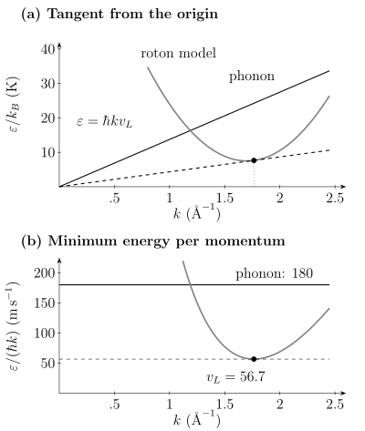
The illustrative spectrum of exercise 2 has a phonon speed of $180\ \mathrm{m\,s^{-1}}$ and a lower roton Landau speed of $56.7\ \mathrm{m\,s^{-1}}$. The tangent touches at $k_*>k_0$: minimizing energy is different from minimizing energy divided by momentum. These are model curves, not a fit to a particular helium sample.

The bound tests energetic emission into the stated spectrum. An aperture, rough wall or weak link may nucleate vortices at a lower speed. Heating, dynamical instability and phase slips can also limit observed flow. Thus a measured threshold below $v_L$ need not contradict the spectrum. On a lattice or with a synthetic gauge field, analyze the actual current-carrying state’s excitation spectrum; crystal momentum cannot simply be substituted into the Galilean argument.

Quantized circulation and rotation

For a scalar component, with no applied gauge source and a closed contour avoiding vortex cores,

$$\oint_{\mathcal C}\mathbf v_s\cdot d\boldsymbol\ell =\ell\frac{h}{M},\qquad \ell\in\mathbb Z.$$

A thin annulus of radius $R$ in winding sector $\ell$ therefore has $v_\ell=\ell\hbar/(MR)$. Quantization fixes allowed circulations; barriers to vortex crossings and phase slips determine their lifetimes. The energy density is $\rho_s v_\ell^2/2$, not the condensate density times the single-atom kinetic energy.

Coarse-grained steady rotation at angular speed $\Omega>0$ gives, for ordinary aligned singly quantized vortices,

$$n_v=\frac{2\Omega}{\kappa}=\frac{M\Omega}{\pi\hbar}, \qquad \kappa=\frac hM.$$

This follows by equating the coarse-grained vorticity $n_v\kappa$ to $2\Omega$. Finite-vessel effects, pinning, multiply quantized vortices and multicomponent textures change this simple counting. It is not a formula for an arbitrary nonequilibrium vortex tangle.

Two-dimensional films and finite observation scales

For an equilibrium two-dimensional scalar fluid with ordinary integer vortices in the BKT regime, the long-distance renormalized stiffness satisfies

$$\begin{aligned} \Upsilon_R(T_{\rm BKT}^-)&=\frac{2k_BT_{\rm BKT}}{\pi},\\ \rho_s^{2D}(T_{\rm BKT}^-)&=\frac{2M^2k_BT_{\rm BKT}}{\pi\hbar^2}. \end{aligned}$$

The second expression is a mass per area. For positive diagonal anisotropic stiffnesses, the spatially rescaled criterion uses $\sqrt{\Upsilon_x\Upsilon_y}$. A bare microscopic stiffness, or a finite-frequency effective stiffness, is not automatically the long-distance quantity in this formula.

For example, at $T=0.70\ \mathrm K$ and $M=m_4=6.646\times10^{-27}\ \mathrm{kg}$, the universal-line values are

$$\begin{aligned} \frac{\Upsilon_R}{k_B}&=0.446\ \mathrm K,\\ n_s^{2D}&=3.68\ \mathrm{nm^{-2}},\\ \rho_s^{2D}&=2.45\times10^{-8}\ \mathrm{kg\,m^{-2}}. \end{aligned}$$

These are comparison values, not densities established merely by observing a rounded crossing. In a finite-frequency experiment, vortices explore only a finite distance within a cycle. Larger samples and slower measurements can therefore give different effective stiffnesses. The solved film example below shows why a common trend can still be statistically unresolved.

Porous media and substrates add further physics: dead layers, tortuosity, weak links and mechanical loading can separate local coherence from sample-scale response. A torsional oscillator senses the loaded cell; changes in elasticity or viscoelastic coupling can mimic part of a decoupling signal. Trapped or driven fluids need their own response model. Equilibrium BKT and two-fluid formulas cannot be transferred unchanged to an open polariton or magnon system.

A helium sound estimate

At $1.60\ \mathrm K$ and saturated vapor pressure, the Donnelly–Barenghi compilation gives $\rho_s/\rho\simeq0.838$ and a fountain-pressure entropy $\bar s\simeq281.5\ \mathrm{J\,kg^{-1}K^{-1}}$. Its saturated-path heat capacity is about $6.29\ \mathrm{J\,mol^{-1}K^{-1}}$, or $1.57\ \mathrm{kJ\,kg^{-1}K^{-1}}$. At this low vapor pressure it is a useful approximation to $c_p$ for the simple estimate

$$\begin{aligned} c_{2,\rm est} &=\left[\frac{0.838}{0.162} \frac{1.60(281.5)^2}{1.57\times10^3}\right]^{1/2} \mathrm{m\,s^{-1}}\\ &\simeq20.4\ \mathrm{m\,s^{-1}}. \end{aligned}$$

This is a consistency estimate at the percent level, not an exact inversion for $\rho_s$. A precision comparison uses the full thermodynamic derivatives, heat-capacity convention, measured sound response and uncertainties at the same temperature and pressure. It should not combine a state-specific thermodynamic table with a spectrum whose temperature is unspecified.

Exercises

1. Twist curvature and particle winding

For a rectangular sample let $F(\boldsymbol\varphi)-F(0)=\frac12\sum_iC_i\varphi_i^2$. Find $\Upsilon_{ii}$ and $\rho^s_{ii}$. Then suppose atomic paths are grouped into tightly bound pairs: $N_a=2N_p$, $M_p=2m_a$, and a pair winding has $W_a=2W_p$. Show that the winding estimate is consistent when all three changes are made.

Solution

The curvature gives

$$\Upsilon_{ii}=\frac{L_i^2}{V}C_i, \qquad \rho^s_{ii}=\frac{M^2}{\hbar^2}\Upsilon_{ii}$$

for the chosen coherent phase and carrier mass. In three dimensions the units are $\mathrm{J\,m^{-1}}$ and $\mathrm{kg\,m^{-3}}$ respectively. Atomic and pair winding descriptions agree because

$$\frac{m_a}{N_a}\langle W_a^2\rangle =\frac{m_a}{2N_p}\,4\langle W_p^2\rangle =\frac{M_p}{N_p}\langle W_p^2\rangle.$$

The grouping is a model assumption about bound paths, not an instruction to relabel an arbitrary interacting path ensemble. A pair phase twist is also twice the atomic phase twist under the same physical boost; its free-energy curvature changes accordingly.

2. Phonon–roton Landau bound

Use the illustrative isotropic branches

$$\begin{aligned} \varepsilon_{\rm ph}(k)&=\hbar ck,\\ \varepsilon_{\rm rot}(k)&=\Delta+\frac{\hbar^2(k-k_0)^2}{2\mu_*}, \end{aligned}$$

with $c=180\ \mathrm{m\,s^{-1}}$, $\Delta/k_B=7.5\ \mathrm K$, $k_0=1.70\ \text{Å}^{-1}$ and $\mu_*=0.18m_4$. Minimize $\varepsilon/(\hbar k)$ over both branches. Does an aperture threshold of $15\ \mathrm{m\,s^{-1}}$ contradict this model?

Solution

The phonon ratio is $c$. The roton ratio is stationary when $k\varepsilon'(k)=\varepsilon(k)$, giving

$$k_*^2=k_0^2+\frac{2\mu_*\Delta}{\hbar^2}, \qquad k_*\simeq1.764\ \text{Å}^{-1}.$$

At the minimum, phase and group velocities coincide:

$$\begin{aligned} v_L^{\rm rot}&=\frac{\varepsilon(k_*)}{\hbar k_*}\\ &=\frac{\hbar(k_*-k_0)}{\mu_*}\\ &\simeq56.7\ \mathrm{m\,s^{-1}}. \end{aligned}$$

This is lower than $180\ \mathrm{m\,s^{-1}}$ and controls the two-branch result. The parabolic approximation must remain valid around $k_*$ when applied to a real spectrum. The smaller aperture threshold may reflect vortex nucleation or heating rather than homogeneous quasiparticle emission; compare local flow speed, geometry and temperature before attributing the onset.

3. Phonons and the low-temperature second sound

Derive the normal density for one isotropic branch $\varepsilon(p)=cp$ in three dimensions. Using its energy density $u=\pi^2(k_BT)^4/(30\hbar^3c^3)$, show that the negligible-expansion second-sound formula tends to $c/\sqrt3$ as $\rho_n/\rho\to0$ within the hydrodynamic regime.

Solution

Isotropy and $x=\beta cp$ give

$$\rho_n=\frac{1}{6\pi^2\hbar^3\beta^4c^5} \int_0^\infty dx\,x^4\frac{e^x}{(e^x-1)^2}.$$

Expanding $e^x/(e^x-1)^2=\sum_{n\ge1}n e^{-nx}$ makes the integral $24\sum_{n\ge1}n^{-4}=4\pi^4/15$. Therefore

$$\rho_n=\frac{2\pi^2}{45}\frac{(k_BT)^4}{\hbar^3c^5} =\frac{4u}{3c^2}.$$

For the phonon gas, $s=4u/(3T)$ and the heat capacity per mass is $c_v=4u/(\rho T)$. With negligible thermal expansion and $\rho_s\simeq\rho$,

$$c_2^2\simeq\frac{\rho}{\rho_n} \frac{T[s/\rho]^2}{c_v} =\frac{4u}{9\rho_n}=\frac{c^2}{3}.$$

The limit is thermodynamic; a finite experiment may become collisionless at very low temperature as the phonon mean free path grows. That can prevent observation of hydrodynamic second sound even though the formal limiting speed is finite.

4. A finite-frequency film comparison

Synthetic fits of $\Upsilon_{\rm eff}/k_B$ to $2T/\pi$ give the candidate crossing temperatures below. Treat the listed one-standard-deviation errors as independent for this exercise. What do the size and frequency differences establish?

Cell side	100 Hz	1000 Hz
$2\ \mathrm{mm}$	$0.702\pm0.006\ \mathrm K$	$0.713\pm0.008\ \mathrm K$
$8\ \mathrm{mm}$	$0.700\pm0.005\ \mathrm K$	$0.707\pm0.007\ \mathrm K$

Solution

The smaller-minus-larger-cell differences are $0.002\pm0.008\ \mathrm K$ at 100 Hz and $0.006\pm0.011\ \mathrm K$ at 1000 Hz. The high-minus-low-frequency differences are $0.011\pm0.010\ \mathrm K$ and $0.007\pm0.009\ \mathrm K$. Uncertainties follow by adding independent variances; shared calibration errors would require their covariances instead.

The common upward trend with frequency is consistent with a shorter distance explored during a cycle, but none of these differences is individually resolved. The data describe a finite-scale BKT-compatible crossover. More sizes, lower frequencies and a mechanical model of the substrate are needed to estimate a thermodynamic transition. Agreement with the universal line alone does not exclude viscoelastic or inhomogeneity effects.

5. Circulation and the energy of an annulus

Take $^4$He in a thin annulus of radius $R=1.0\ \mathrm{cm}$ and winding $\ell=3$. Find the circulation, speed and flow energy per total atom when $\rho_s/\rho=f_s$. What vortex density corresponds to rigid rotation at $\Omega=1.0\ \mathrm{s^{-1}}$ in a large vessel?

Solution

Using $m_4=6.646\times10^{-27}\ \mathrm{kg}$,

$$\begin{aligned} \oint\mathbf v_s\cdot d\boldsymbol\ell &=\frac{3h}{m_4}\\ &\simeq2.99\times10^{-7}\ \mathrm{m^2\,s^{-1}},\\ v_3&\simeq4.76\times10^{-6}\ \mathrm{m\,s^{-1}}. \end{aligned}$$

The total kinetic energy divided by the total atom number is

$$\frac{E_{\rm flow}}{N}=f_s\frac{m_4v_3^2}{2} \simeq f_s\,7.5\times10^{-38}\ \mathrm J.$$

It is weighted by the superfluid fraction, not by the condensate fraction. For aligned singly quantized vortices, $n_v=m_4\Omega/(\pi\hbar)\simeq2.0\times10^7\ \mathrm{m^{-2}}$. Neither integer circulation nor this rotation count determines a phase-slip lifetime.

References

• R. J. Donnelly and C. F. Barenghi, “The Observed Properties of Liquid Helium at the Saturated Vapor Pressure,” Journal of Physical and Chemical Reference Data 27, 1217–1274 (1998), doi:10.1063/1.556028.
• R. J. Donnelly, Quantized Vortices in Helium II, Cambridge University Press (1991).
• M. E. Fisher, M. N. Barber, and D. Jasnow, “Helicity Modulus, Superfluidity, and Scaling in Isotropic Systems,” Physical Review A 8, 1111–1124 (1973), doi:10.1103/PhysRevA.8.1111.
• I. M. Khalatnikov, An Introduction to the Theory of Superfluidity, W. A. Benjamin (1965).
• L. D. Landau, “The Theory of Superfluidity of Helium II,” Physical Review 60, 356–358 (1941), doi:10.1103/PhysRev.60.356.
• A. J. Leggett, “Superfluidity,” Reviews of Modern Physics 71, S318–S323 (1999), doi:10.1103/RevModPhys.71.S318.
• D. R. Nelson and J. M. Kosterlitz, “Universal Jump in the Superfluid Density of Two-Dimensional Superfluids,” Physical Review Letters 39, 1201–1205 (1977), doi:10.1103/PhysRevLett.39.1201.
• O. Penrose and L. Onsager, “Bose–Einstein Condensation and Liquid Helium,” Physical Review 104, 576–584 (1956), doi:10.1103/PhysRev.104.576.
• L. P. Pitaevskii and S. Stringari, “Second Sound in Ultracold Atomic Gases,” preprint (2015), arXiv:1510.01306.
• L. Pitaevskii and S. Stringari, Bose–Einstein Condensation and Superfluidity, Oxford University Press (2016).
• E. L. Pollock and D. M. Ceperley, “Path-Integral Computation of Superfluid Densities,” Physical Review B 36, 8343–8352 (1987), doi:10.1103/PhysRevB.36.8343.
• D. Vollhardt and P. Wölfle, The Superfluid Phases of Helium 3, Dover (2013).