Magnetic Moments in Matter

A magnetic moment quoted for a material is not one context-free number. A Curie–Weiss fit, a high-field magnetization curve, magnetic diffraction, and an energy-integrated spectrum answer different operator, state, and resolution questions. Their answers can disagree even when every measurement and model is correct.

The connection is the physical magnetic-moment operator. Projecting it into a crystal-field doublet explains an anisotropic response; comparing its mean, variance, and thermal susceptibility explains why different experiments quote different moments. A low-energy spin model is useful when its states and operators reproduce the observables within the energy range being studied.

Required background. Magnetic Moments and g-Factors supplies magnetic-moment signs, magnetons, Zeeman conventions, and Landé algebra.

Helpful background. Hund’s Rules supplies the free-ion baseline. Spin–Orbit Coupling in Solids explains crystal-field, covalency, and spin–orbit projection. Magnetic Susceptibility explains Curie and high-field measurements, while Itinerant Magnetism explains distributed and scale-dependent electronic moments.

Magnetic-moment units and physical operators

A sample magnetic dipole moment $m$ in $\mathrm{A\,m^2}$ becomes a magnetization $M=m/V$ in $\mathrm{A/m}$ after division by sample volume. A value in $\mu_B$ per formula unit becomes a moment per magnetic ion only after accounting for the number and occupancy of those ions. Squared moments, which add in spectral sum rules, instead have units of $\mu_B^2$.

The operator also matters. A spin-only moment inside an atomic sphere excludes orbital, ligand, and interstitial contributions that a bulk measurement may include. First ask which magnetic density the number describes, then which state and measurement determine it.

Free-Ion Baselines Are Starting Points

For an isolated, isotropic angular-momentum multiplet with quantum number $J$ and Landé factor $g_J$, two standard scales are

$$\mu_{\mathrm{eff}} = g_J\sqrt{J(J+1)}\,\mu_B$$

and

$$\mu_{\mathrm{sat}} = g_JJ\,\mu_B.$$

The first is the Curie fluctuation scale of a thermally randomized multiplet. The second is its maximum moment along a quantization axis. They differ even for an ideal ion because $\sqrt{J(J+1)}\ne J$. Magnetic Susceptibility develops the Curie–Weiss fit and its SI–cgs, background, and fit-window controls.

Hund’s Rules may supply an approximate free-ion term, but a crystal is not a free ion. Crystal fields split the multiplet, covalency moves magnetic density onto ligands, spin–orbit coupling changes the active basis, and exchange or hybridization can mix nominal configurations. A free-ion moment is therefore a baseline to test, not a value to impose on a solid.

“Orbital quenching” also needs care. A nondegenerate real crystal-field state can have vanishing first-order $\langle\mathbf L\rangle$, while virtual excited states still generate anisotropic $g$ factors, Van Vleck response, and anisotropy. Magnetic Moments from Orbital Motion derives the bare current-loop moment. The crystalline material problem begins after local symmetry and hybridization have changed that atomic basis.

Project the Physical Moment into the Retained Subspace

Let $P$ project onto a selected low-energy manifold. If an orthonormal frame is stored as the columns of $U$, then

$$P = UU^\dagger, \qquad U^\dagger U = I.$$

Changing the frame by $U\mapsto UV$ with unitary $V$ does not change $P$. The projected Hamiltonian and every physical operator must be rotated in the same frame. Projecting only the Hamiltonian while continuing to use a bare-spin operator is not a consistent effective theory.

For a time-reversal-invariant Kramers doublet, choose a dimensionless pseudospin $\widetilde{\mathbf s}=\boldsymbol\sigma/2$. The physical moment in retained coordinates is

$$\hat\mu_\alpha^{\mathrm{eff}} = U^\dagger\hat\mu_\alpha U = -\mu_B \sum_\beta g_{\alpha\beta} \widetilde s_\beta.$$

Its lifted full-space restriction is $P\hat\mu_\alpha P=U\hat\mu_\alpha^{\mathrm{eff}}U^\dagger$. Here $\alpha$ labels a laboratory-space component and $\beta$ a pseudospin-frame component. This distinction keeps the full-space projector separate from its matrix in the retained coordinate frame.

The identity component vanishes because the moment is odd under time reversal while the two states form a Kramers pair. A generic projected subspace, or a subspace selected after time reversal is broken, may allow an identity offset. The Pauli matrices label the doublet; they are not automatically the matrices of bare electron spin, orbital angular momentum, or total $\mathbf J$.

A time-reversal-symmetric non-Kramers doublet has a different operator structure. In a basis where time reversal acts as complex conjugation, only one Pauli direction is time-reversal odd; point-group symmetry can restrict that magnetic dipole component further. The remaining pseudospin components are time-reversal even and may represent quadrupoles or higher multipoles. A three-component Kramers $g$-tensor description is therefore not universal. A nonmagnetic singlet can likewise have no permanent moment yet retain a finite Van Vleck response through virtual excited states. Rau and Gingras review these different rare-earth low-energy degrees of freedom.

The effective Zeeman Hamiltonian in retained coordinates is

$$H_Z^{\mathrm{eff}} = \mu_B \mathbf B^{\mathsf T} \mathbf g \widetilde{\mathbf s}.$$

In the original Hilbert space, $PH_ZP=UH_Z^{\mathrm{eff}}U^\dagger$.

For a field $\mathbf B=B\mathbf n$, the doublet splitting is

$$\Delta E(\mathbf n) = \mu_BB \sqrt{ \mathbf n^{\mathsf T} \mathbf G \mathbf n }, \qquad \mathbf G = \mathbf g\mathbf g^{\mathsf T}.$$

A pseudospin-basis rotation changes the displayed matrix $\mathbf g$ but leaves $\mathbf G$ and the splitting invariant. Chibotaru, Ceulemans, and Bolvin discuss how symmetry and continuity constrain choices of the tensor. Relative signs and the full operator matrices can still matter when the moment is combined with exchange, neutron matrix elements, or another projected operator. Spin–Orbit Coupling in Solids explains how the crystal-field and spin–orbit states that define $P$ are obtained.

Five Moment Measures Are Not One Number

Curie-effective moment

For a degenerate projected spin $\widetilde S$ in a weak-field, high-temperature window above its interactions but below discarded levels, let $\nu$ be the number of identical active moments per formula unit. Per mole of formula units, the SI Curie tensor for susceptibility differentiated with respect to internal $\mathbf H$ is

$$C_{\alpha\beta}^{\mathrm{mol}} = \frac{ \mu_0N_A\nu\mu_B^2 }{3k_B} \widetilde S(\widetilde S+1) G_{\alpha\beta}.$$

For a mole of active moment centers, or one center per formula unit, set $\nu=1$. A diluted or partially occupied sublattice requires its measured concentration rather than silently using this value. The expression uses $\mathbf B\simeq\mu_0\mathbf H_{\mathrm{int}}$ in the weak-response regime; demagnetizing and local-field corrections belong in the experimental forward model. For the doublet defined above, $\widetilde S=1/2$; a larger retained multiplet requires its own dimensionless spin matrices.

Along a unit vector $\mathbf n$, this corresponds to

$$\mu_{\mathrm{eff},\mathbf n}^2 = \mu_B^2 \widetilde S(\widetilde S+1) \mathbf n^{\mathsf T}\mathbf G\mathbf n.$$

This is a susceptibility coefficient, not a static expectation value. Excited crystal-field states, Van Vleck terms, exchange, Kondo physics, impurity tails, or a poor temperature window invalidate the simple identification.

Nor is a quantum static susceptibility generally just an ordinary equal-time variance. When $[\hat H,\hat\mu_\alpha]\ne0$, the equilibrium response uses the Kubo–Mori imaginary-time covariance. Equal-time fluctuations, thermodynamic response, and detector-bandwidth noise coincide only in stated commuting, classical, and limit conventions. Fluctuations and Susceptibilities derives that distinction.

Saturation moment

For an isolated doublet that remains valid to the applied field, the longitudinal saturated moment is

$$\mu_{\mathrm{sat},\mathbf n} = \frac{\mu_B}{2} \sqrt{ \mathbf n^{\mathsf T} \mathbf G \mathbf n }.$$

An anisotropic $g$ tensor can make the physical moment nonparallel to the field. Level mixing, metamagnetic transitions, unsaturated itinerant polarization, and sample heating can all prevent a measured high-field value from reaching this ideal limit.

Ordered moment

An ordered moment is the symmetry-selected static expectation of the physical moment density in a declared magnetic basis. It may be uniform or occur at a finite propagation vector. Quantum and thermal fluctuations, covalency, itinerancy, canting, and domain averaging can reduce its reported value. A finite-system symmetric eigenstate can have zero one-point expectation even when correlations diagnose incipient order.

Equal-time local moment

For one declared local operator, the instantaneous second moment is

$$m_{\mathrm{inst}}^2 = \left\langle \hat{\boldsymbol\mu}_i \cdot \hat{\boldsymbol\mu}_i \right\rangle.$$

This can remain large without long-range order. In an itinerant calculation, the word “local” additionally requires a region, orbital projector, or Wannier space; different defensible partitions need not give the same number.

Fluctuating moment

With $\delta\hat{\boldsymbol\mu}_i=\hat{\boldsymbol\mu}_i- \langle\hat{\boldsymbol\mu}_i\rangle$, define

$$m_{\mathrm{fluc}}^2 = \left\langle \delta\hat{\boldsymbol\mu}_i \cdot \delta\hat{\boldsymbol\mu}_i \right\rangle.$$

For the same operator, state, site, and normalization,

$$m_{\mathrm{inst}}^2 = m_{\mathrm{mean}}^2 + m_{\mathrm{fluc}}^2, \qquad m_{\mathrm{mean}}^2 = \left| \left\langle \hat{\boldsymbol\mu}_i \right\rangle \right|^2.$$

The mean contains field-induced polarization as well as spontaneous order. It may be called $m_{\mathrm{ord}}$ only in a source-selected zero-field ordered state with the same site, sublattice, and domain convention. For noncollinear, multi-sublattice, or multi-$\mathbf Q$ order, the corresponding statement uses the complete elastic Fourier weight rather than one scalar ordered moment. The identity is exact only when the static and connected pieces refer to the same physical operator and state. Combining a bulk Curie fit, a site-projected calculation, and a resolution-limited neutron integral does not automatically satisfy it.

Projection changes the total spectral weight

A low-energy moment operator describes transitions within the retained subspace. Its square need not equal the projection of the full squared moment. For a Hermitian component and the frame $U$ above,

$$\begin{aligned} U^\dagger\hat\mu_\alpha^2U -\bigl(U^\dagger\hat\mu_\alpha U\bigr)^2 &=U^\dagger\hat\mu_\alpha(1-P)\hat\mu_\alpha U\\ &\succeq0. \end{aligned}$$

To see the sign, write the right side as $X^\dagger X$ with $X=(1-P)\hat\mu_\alpha U$. It counts transition matrix elements from the retained states to discarded states. These transitions contribute to a full frequency integral even when the discarded levels have negligible thermal population. Thus the doublet’s $g$ tensor can correctly predict low-energy spectral weight while underestimating the full equal-time squared moment. The Ce example below makes the difference explicit.

Elastic and Inelastic Weight Share a Sum Rule

Use the normalized Fourier operator

$$\hat\mu_{\mathbf q}^\alpha = \frac{1}{\sqrt N} \sum_j e^{-i\mathbf q\cdot\mathbf R_j} \hat\mu_j^\alpha$$

and the angular-frequency convention

$$S_\mu^{\alpha\beta}(\mathbf q,\omega) = \frac{1}{2\pi} \int_{-\infty}^{\infty}dt\, e^{i\omega t} \left\langle \hat\mu_{\mathbf q}^\alpha(t) \hat\mu_{-\mathbf q}^\beta(0) \right\rangle.$$

For $N$ equivalent sites on a Bravais lattice, summing all $N$ wavevectors in its Brillouin zone and all frequencies gives

$$\frac{1}{N} \sum_{\mathbf q,\alpha} \int_{-\infty}^{\infty}d\omega\, S_\mu^{\alpha\alpha}(\mathbf q,\omega) = m_{\mathrm{inst}}^2.$$

The disconnected elastic contribution carries the static mean, which may be field induced or ordered; the connected elastic and inelastic contributions carry fluctuations. Structure Factors gives the general correlation-function derivation, while Neutron Scattering explains polarization factors, magnetic form factors, absolute normalization, background, and resolution.

A real experiment covers a finite region of $\mathbf q$ and $\omega$. Missing weight may be elastic, above the incident-energy window, hidden by a phonon or background, transferred to ligand magnetization, or carried by degrees of freedom outside a spin-only model. A partial integral is evidence about that window, not a proof that the remaining moment has vanished. Lorenzana, Seibold, and Coldea discuss this distinction for cuprate neutron spectra.

Local and Itinerant Are Scale-Dependent Limits

An ion-centered moment can be useful at short times while the same material has coherent itinerant quasiparticles at low energy. Conversely, a metal can contain localized rare-earth or impurity moments carried by electrons distinct from its Fermi surface. The useful question is not whether the material is permanently “local” or “itinerant,” but which variables retain their amplitude over the declared energy, temperature, and length window.

Itinerant Magnetism explains band reconstruction, longitudinal fluctuations, the Stoner continuum, and the Rhodes–Wohlfarth diagnostic. A large Curie-effective moment together with a small spontaneous or saturation moment can support an itinerant or mixed interpretation, but it is not a binary theorem. Crystal-field population, orbital terms, Kondo screening, incomplete saturation, and fit backgrounds can produce similar ratios.

Spatial decomposition is also model dependent. A moment integrated inside an atomic sphere, assigned to a Wannier orbital, or reported on a ligand cluster depends on that partition. The total sample dipole and bulk magnetization are physical, and a spin-density observable can be defined with a specified operator and resolution. A unique atom-by-atom division, especially of orbital magnetization, generally is not. From Quantum Mechanics to Materials explains how the choice of local orbitals affects a material model.

Bulk crystalline orbital magnetization is likewise not generally the sum of site-local $\langle\mathbf L\rangle$. It can include itinerant circulation and Berry-geometric contributions from occupied Bloch states, as developed by Xiao, Chang, and Niu. An atomic orbital moment remains a useful local diagnostic only when its projection and scope are declared.

When a fixed-length model is reliable

A spin or pseudospin Hamiltonian describes a stable low-energy multiplet when charge excitations, higher crystal-field states, and longitudinal amplitude modes are well separated from exchange, thermal, and Zeeman energies. The probe must also stay within the range represented by that model. All physical operators must be projected consistently; virtual transitions can produce additional corrections to both the Hamiltonian and observables.

Compare the predicted directional susceptibility, saturation, and subgap spectral intensities. Agreement with an energy dispersion alone does not check the moment matrix elements. If a nearby level mixes strongly, magnetic density moves onto ligands, or low-energy longitudinal fluctuations change the moment’s length, include those degrees of freedom. Exchange Interactions and Common Spin Hamiltonians describe interactions once the retained variables have been identified.

Worked example: an anisotropic Kramers doublet

Consider a hypothetical tetragonal Ce$^{3+}$ insulator. The free-ion baseline has $J=5/2$ and $g_J=6/7$. In this idealized example, a crystal field isolates a pure $|m_J=\pm1/2\rangle$ ground doublet by $\Delta_{\mathrm{CF}}=18\,\mathrm{meV}$. In its principal axes the projected tensor is

$$\mathbf g = \operatorname{diag} \left( \frac{18}{7}, \frac{18}{7}, \frac{6}{7} \right).$$

Take one Ce ion per formula unit, neglect covalency, and use dimensionless $J$ matrices in $\hat{\boldsymbol\mu}=-g_J\mu_B\hat{\mathbf J}$. The $z$ axis is tetragonal and $x,y$ lie in the basal plane. Within the states $|m_J=\pm1/2\rangle$, the matrix element $\langle+1/2|J_+|-1/2\rangle=3$ gives $J_x=3\widetilde s_x$, $J_y=3\widetilde s_y$, and $J_z=\widetilde s_z$, explaining the tensor above.

Suppose exchange is below $0.06\,\mathrm{meV}$. At $5\,\mathrm K$, $k_BT\simeq0.43\,\mathrm{meV}$; the largest splitting at $5\,\mathrm T$ is $0.74\,\mathrm{meV}$. Both are well below the $18\,\mathrm{meV}$ gap. A weak-field Curie fit over $5$–$15\,\mathrm K$ can then resolve the doublet contribution after allowing for a Van Vleck background. Spectroscopy below $2\,\mathrm{meV}$ probes its low-energy sector, while higher-energy spectroscopy tests the discarded levels.

The free-ion numbers are

$$\mu_{\mathrm{eff}}^{\mathrm{ion}} = \frac67\sqrt{\frac{35}{4}}\,\mu_B \simeq 2.54\,\mu_B$$

and

$$\mu_{\mathrm{sat}}^{\mathrm{ion}} = \frac67\frac52\,\mu_B \simeq 2.14\,\mu_B.$$

Inside the doublet, the zero-temperature asymptotic basal and axial saturation moments are instead

$$\mu_{\mathrm{sat},\perp} = \frac97\,\mu_B \simeq 1.29\,\mu_B, \qquad \mu_{\mathrm{sat},\parallel} = \frac37\,\mu_B \simeq 0.43\,\mu_B.$$

The corresponding isolated-doublet directional Curie-effective coefficients are about $2.23\,\mu_B$ and $0.74\,\mu_B$, and the ideal powder root-mean-square value is $1.87\,\mu_B$. They apply only in the weak-field window above the interaction scale and below the crystal-field gap. Likewise, $5\,\mathrm T$ at $5\,\mathrm K$ need not realize the asymptotic saturation moments quoted above. At temperatures or fields that populate or admix the next doublet, the rank-two projection must be reopened.

For this example, projection also changes the integrated moment-squared weight:

$$\begin{aligned} \langle\hat{\boldsymbol\mu}^{2}\rangle &=g_J^2J(J+1)\mu_B^2=\frac{315}{49}\,\mu_B^2,\\ \sum_\alpha\langle(\hat\mu_\alpha^{\mathrm{eff}})^2\rangle &=\frac{\operatorname{Tr}\mathbf G}{4}\mu_B^2 =\frac{171}{49}\,\mu_B^2. \end{aligned}$$

The difference, $144\mu_B^2/49$, is carried by transitions to higher crystal-field states. These equalities hold for any state supported entirely within this ideal ground doublet. The full moment has magnitude $\sqrt{315/49}\,\mu_B\simeq2.54\,\mu_B$, even though the doublet-only powder Curie scale is $\sqrt{171/49}\,\mu_B\simeq1.87\,\mu_B$. The two numbers refer to different transition sets.

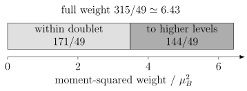
In the ideal Ce doublet, $171/49$ of the moment-squared weight remains within the doublet and $144/49$ connects it to higher levels, in units of $\mu_B^2$. Low thermal population of those higher levels does not remove their transition weight from the full sum rule.

Worked example: compare moments from different probes

Consider a hypothetical correlated metal with one transition-metal site per formula unit. The reported data are a Curie-effective moment $3.10\,\mu_B$, an extrapolated high-field moment $1.05\,\mu_B$, a diffraction ordered moment $0.65\,\mu_B$, an absolutely normalized equal-time $m_{\mathrm{inst}}=2.60\,\mu_B$ reported from a converged neutron integral, and a spin-density calculation reporting $0.80\,\mu_B$ inside one atomic sphere.

The Curie fit uses $180$–$350\,\mathrm K$, whereas the high-field magnetization is measured at $2\,\mathrm K$. The diffraction and neutron numbers refer to the same $2\,\mathrm K$ zero-measurement-field ordered state and domain. They use the same full formula-unit magnetic operator and include all magnetic components. The neutron integral includes the full Brillouin zone, elastic scattering, negative frequencies through detailed balance, and an energy range whose tail has converged. In contrast, the atomic-sphere calculation includes only spin density and omits ligand and interstitial contributions.

For the same complete local operator, the connected fluctuation scale would be

$$m_{\mathrm{fluc}} = \sqrt{ (2.60\,\mu_B)^2 - (0.65\,\mu_B)^2 } \simeq 2.52\,\mu_B.$$

Here the static mean is the ordered moment because the state and domain are the same. A finite energy window or a different spatial partition would invalidate this exact subtraction. The high-temperature Curie coefficient and the atomic-sphere result cannot be substituted into it.

Substantial instantaneous magnetic weight can therefore coexist with a much smaller ordered moment. This hierarchy alone does not determine one spin quantum number or prove a rigid local-spin model.

Exercises

1. Read an anisotropic g tensor

A Kramers doublet has $\mathbf g=\operatorname{diag}(2.4,1.2,0.6)$. A field points along $\mathbf n=(1,1,0)/\sqrt2$. Find the splitting per unit field, the longitudinal saturated moment, and the powder Curie-effective coefficient. Show that a pseudospin-basis rotation $\mathbf g\mapsto\mathbf g\mathbf R$ with a proper rotation $\mathbf R\in SO(3)$ changes none of these quantities.

Solution

Here

$$\mathbf n^{\mathsf T}\mathbf G\mathbf n = \frac{2.4^2+1.2^2}{2} = 3.60.$$

Therefore

$$\frac{\Delta E}{B} = \sqrt{3.60}\,\mu_B \simeq 1.90\,\mu_B,$$

where the right-hand side has the units of magnetic moment. The saturated longitudinal moment is half that value, about $0.95\,\mu_B$. The full moment vector need not be parallel to the field. For $\widetilde S=1/2$, the powder coefficient satisfies

$$\mu_{\mathrm{eff,powder}}^2 = \mu_B^2 \frac{\widetilde S(\widetilde S+1)}{3} \operatorname{Tr}\mathbf G = 1.89\,\mu_B^2,$$

so $\mu_{\mathrm{eff,powder}}\simeq1.37\,\mu_B$. Under the basis rotation,

$$\mathbf G' = (\mathbf g\mathbf R)(\mathbf g\mathbf R)^{\mathsf T} = \mathbf g\mathbf R\mathbf R^{\mathsf T}\mathbf g^{\mathsf T} = \mathbf G.$$

Directional splittings, saturation moments, and the powder trace are therefore invariant even though the displayed $\mathbf g$ matrix changes.

2. Convert a sample moment to microscopic units

A $4.0\,\mathrm{mg}$ crystal of molar mass $400\,\mathrm{g\,mol^{-1}}$ contains two equivalent magnetic ions per formula unit and four formula units per crystallographic cell. Its background-corrected saturated sample moment is $1.79\times10^{-4}\,\mathrm{A\,m^2}$. Find the moment per formula unit and per magnetic ion in $\mu_B$, per cell in $\mu_B$, and per mole of formula units in $\mathrm{A\,m^2\,mol^{-1}}$. State what additional information is needed to quote magnetization in $\mathrm{A/m}$.

Solution

The sample contains

$$n = \frac{4.0\times10^{-3}\,\mathrm g} {400\,\mathrm{g\,mol^{-1}}} = 1.0\times10^{-5}\,\mathrm{mol}$$

of formula units. The number of formula units is $nN_A$. Thus

$$\mu_{\mathrm{f.u.}} = \frac{1.79\times10^{-4}\,\mathrm{A\,m^2}} {(1.0\times10^{-5})N_A} \simeq 3.21\,\mu_B.$$

With two fully occupied equivalent magnetic sites, the value is $1.60\,\mu_B$ per ion. Four formula units give $12.8\,\mu_B$ per cell when calculated before rounding. The molar dipole moment is

$$m_{\mathrm{mol}} = (3.21\,\mu_B)N_A \simeq 17.9\,\mathrm{A\,m^2\,mol^{-1}}.$$

The sample volume, including the convention for porosity or packing if relevant, is needed for $M=m/V$ in $\mathrm{A/m}$.

3. Balance elastic and inelastic weight

For one consistently normalized local operator in a source-selected zero-field ordered state with a single declared sublattice and domain, $m_{\mathrm{inst}}=2.40\,\mu_B$ and $m_{\mathrm{ord}}=0.80\,\mu_B$. Find the connected fluctuating moment. If an experiment captures $70\%$ of its connected spectral weight, what moment scale would that partial integral report?

Solution

The complete connected variance is

$$m_{\mathrm{fluc}} = \sqrt{2.40^2-0.80^2}\,\mu_B = \sqrt{5.12}\,\mu_B \simeq 2.26\,\mu_B.$$

Spectral weights add as squared moments, so the partial integral reports

$$m_{\mathrm{partial}} = \sqrt{0.70}\,m_{\mathrm{fluc}} \simeq 1.89\,\mu_B.$$

The remaining weight is not automatically absent; it may lie outside the measured momentum, energy, polarization, or elastic window.

4. Test the separation of energy scales

A candidate doublet is separated by $12\,\mathrm{meV}$ from the next level. The working window has exchange $4\,\mathrm{meV}$, maximum Zeeman energy $3.5\,\mathrm{meV}$, probe transfer $5\,\mathrm{meV}$, and $k_BT=2.6\,\mathrm{meV}$. Is a rank-two fixed-length model controlled? What would improve the case?

Solution

The probe reaches about $42\%$ of the gap, while exchange and Zeeman energies are themselves about a third of it. This is not a strong separation of scales. A subgap probe does not by itself populate the higher level, but interactions and fields can mix levels virtually. Include the next level or quantify its corrections before relying on a doublet alone.

Lower temperature and field reduce thermal population and Zeeman mixing, but do not remove the $4\,\mathrm{meV}$ exchange scale. A much larger gap, weaker exchange in a different regime, or an explicit multilevel calculation would improve the case. Even with a strong hierarchy, the projected $g$ tensor and static and subgap dynamic observables must agree.

References

• A. Abragam and B. Bleaney, Electron Paramagnetic Resonance of Transition Ions, Oxford University Press (1970).

• S. Blundell, Magnetism in Condensed Matter, Oxford University Press (2001), doi:10.1093/oso/9780198505921.001.0001.

• L. F. Chibotaru, A. Ceulemans, and H. Bolvin, “Unique Definition of the Zeeman-Splitting g Tensor of a Kramers Doublet,” Physical Review Letters 101, 033003 (2008), doi:10.1103/PhysRevLett.101.033003.

• J. Lorenzana, G. Seibold, and R. Coldea, “Sum Rules and Missing Spectral Weight in Magnetic Neutron Scattering in the Cuprates,” Physical Review B 72, 224511 (2005), doi:10.1103/PhysRevB.72.224511.

• J. G. Rau and M. J. P. Gingras, “Frustrated Quantum Rare-Earth Pyrochlores,” Annual Review of Condensed Matter Physics 10, 357–386 (2019), doi:10.1146/annurev-conmatphys-022317-110520.

• D. Xiao, M.-C. Chang, and Q. Niu, “Berry Phase Effects on Electronic Properties,” Reviews of Modern Physics 82, 1959–2007 (2010), doi:10.1103/RevModPhys.82.1959.