Ferromagnetism

In a conventional ferromagnet, the primary magnetic order is spontaneous uniform magnetization. In a selected thermodynamic state, the magnetic-moment density remains nonzero as the externally applied selecting field is removed:

$$\mathbf M_s \ne \mathbf0.$$

Here uniform identifies the primary order. Ferrimagnets and canted antiferromagnets can also have a uniform component, but their opposing sublattice structure distinguishes them from conventional ferromagnets. The word spontaneous distinguishes the phase from an ordinary paramagnet whose magnetization disappears with the applied field.

Neither word means that every macroscopic specimen behaves as one bar magnet. A low-field sample often divides into domains whose local magnetizations have magnitude $M_s$ but cancel in the spatial average. Hysteresis, remanence, and coercivity then depend on domain-wall motion, defects, shape, and measurement history. They are important material properties, but none is the thermodynamic definition of ferromagnetism.

The material physics joins three questions: how magnetic order emerges, why finite samples form domains, and how their response changes with field and temperature. Spontaneous Symmetry Breaking gives the general phase-selection argument, Magnons derives spin-wave quantization, and Exchange Interactions explains microscopic coupling mechanisms.

Required background. Exchange Interactions supplies coupling signs and microscopic mechanisms, while Order Parameters supplies the source-selected definition of a phase.

Helpful background. Spontaneous Symmetry Breaking develops the thermodynamic-limit logic, and Finite-Temperature Phase Transitions supplies transition and scaling caveats.

Magnetization as the Order Parameter

The SI magnetization is magnetic dipole moment per volume:

$$\widehat{\boldsymbol{\mathcal M}} = \frac{1}{V} \sum_i \widehat{\boldsymbol\mu}_i.$$

It has units of $\mathrm{A/m}$. Spin, orbital angular momentum, and itinerant current can all contribute to $\widehat{\boldsymbol\mu}_i$; a site-local sum is only one representation of the total magnetic moment.

In matter,

$$\mathbf B = \mu_0 \left( \mathbf H+\mathbf M \right)$$

in SI units. The magnetic induction $\mathbf B$, magnetic field $\mathbf H$, and magnetization $\mathbf M$ are distinct quantities. Their separation inside a finite magnet depends on the sample’s demagnetizing field and shape anisotropy.

Spontaneous and saturation magnetization

The spontaneous magnetization $M_s(T)$ is the equilibrium order-parameter magnitude inside a pure, selected domain at zero internal field. The saturation magnetization $M_{\mathrm{sat}}(T,H)$ is the high-field moment after domains align and any remaining canting or moment-amplitude response is suppressed.

They can be close at low temperature in a simple local-moment ferromagnet, but they are not definitions of the same limiting procedure. A high field can continue to polarize itinerant bands, crystal-field levels, paramagnetic impurities, or noncollinear components after domains are already aligned.

The order of limits

Introduce a source through $H_{\mathrm{source}}=-\int_V d^3r\,\mathbf h\cdot\mathbf m(\mathbf r)$. Since $\mathbf m$ is magnetization, $\mathbf h$ has SI units of tesla, and $-\mathbf h\cdot\mathbf m$ is an energy density. A selected spontaneous magnetization is

$$\mathbf M_s = \lim_{\mathbf h\to\mathbf0^+} \lim_{V\to\infty} \left\langle \widehat{\boldsymbol{\mathcal M}} \right\rangle_{\mathbf h}.$$

The thermodynamic limit comes first. In a finite system with exact time-reversal or spin-flip symmetry, an unbiased thermal state can have

$$\left\langle \widehat{\boldsymbol{\mathcal M}} \right\rangle = \mathbf0$$

even when it has strong ferromagnetic correlations. Reversing the limits keeps that symmetric answer and misses phase selection.

Long-range order can instead be diagnosed through correlations:

$$\lim_{|\mathbf r|\to\infty} \left\langle \mathbf m(\mathbf r) \cdot \mathbf m(\mathbf0) \right\rangle = M_s^2$$

in an ideal uniform phase. A symmetric mixture of oppositely magnetized states can have zero one-point function but a nonzero long-distance two-point limit.

Broken Symmetry

For an isotropic exchange Hamiltonian without spin–orbit coupling or field, global spin rotations form an $SO(3)$ symmetry. A ferromagnetic state chooses a direction $\mathbf n$:

$$\mathbf M_s = M_s\mathbf n.$$

Rotations about $\mathbf n$ leave the state invariant, so the symmetry-breaking pattern is

$$SO(3) \longrightarrow SO(2).$$

The order-parameter manifold is

$$\frac{SO(3)}{SO(2)} \simeq S^2.$$

Time reversal changes $\mathbf M_s\to-\mathbf M_s$, so a magnetized state also breaks time reversal. The states $\mathbf n$ and $-\mathbf n$ are symmetry-related members of the same ordered phase when the Hamiltonian has that symmetry.

Crystal anisotropy changes the exact symmetry

Spin–orbit coupling ties the magnetization to the lattice. An easy-axis ferromagnet may have only two low-energy orientations, $+M_s\hat{\mathbf z}$ and $-M_s\hat{\mathbf z}$, related by time reversal. An easy-plane magnet retains an approximate angular degree of freedom within a plane. Cubic anisotropy supplies several crystallographically equivalent easy directions.

The order parameter is still magnetization, but the exact broken group, domain variants, critical universality class, and magnon gap all change. Describing every ferromagnet as exact $SO(3)\to SO(2)$ breaking silently discards the material’s spin–orbit and dipolar energies.

A ferromagnetic finite-size exception

Many symmetry-breaking systems have a unique symmetric finite-size ground state and only develop oriented states through near-degenerate superpositions as volume grows. The isotropic Heisenberg ferromagnet is special: its maximal-total-spin ground multiplet can be exactly degenerate even at finite size, and a fully polarized member already has nonzero magnetization.

This exception does not make phase language unnecessary. Robustness to local perturbations, thermodynamic correlations, finite-temperature order, domains, and response still distinguish a ferromagnetic phase from an accidentally degenerate few-spin system.

Exchange and the Uniform State

Using the convention of Exchange Interactions,

$$H_{\mathrm{ex}} = \sum_{i<j} J_{ij} \mathbf s_i\cdot\mathbf s_j,$$

ferromagnetic couplings have $J_{ij}<0$. Parallel spin correlations lower their bond energy.

A negative nearest-neighbor $J$ is neither necessary nor sufficient for a real material to show simple ferromagnetism:

• longer-range couplings can select a spiral or another wavevector;
• anisotropic exchange can favor noncollinear order;
• frustration can suppress long-range order;
• dimensional fluctuations can destroy finite-temperature continuous order;
• itinerant magnetism may not admit fixed local spins;
• dipolar and anisotropy energies determine the mesoscale texture.

For classical spins on a Bravais lattice, a trial spiral has energy proportional to the Fourier-transformed exchange $J(\mathbf q)$. Its minimum selects the classical ordering wavevector. With several sites per cell, one instead examines an exchange matrix and the constraints on each spin; quantum fluctuations can further change the phase. A conventional ferromagnet orders at

$$\mathbf Q=\mathbf0.$$

This reciprocal-space statement is more general than the sign of one bond.

Landau Description Near the Curie Point

For an easy-axis magnet in zero stress and a uniform approximation, let $M$ denote the signed magnetization along the easy axis. A minimal Landau free-energy density is

$$f(M) = f_0 + \frac{a_0}{2} \left( T-T_C \right) M^2 + \frac{b}{4}M^4 - hM,$$

with $a_0>0$, $b>0$, and the same tesla-valued source $h$. For the intrinsic uniform magnetic free energy one can identify $h=\mu_0H_{\mathrm{int}}$; a finite sample additionally requires its magnetostatic energy. Thus $\partial M/\partial H_{\mathrm{int}}=\mu_0\chi_h$, rather than simply $\chi_h$.

At $h=0$, stationarity gives

$$M \left[ a_0(T-T_C) + bM^2 \right] = 0.$$

The mean-field branches are

$$M_s(T) = \begin{cases} 0, &T>T_C, \\[4pt] \pm \sqrt{ \dfrac{ a_0(T_C-T) }{b} }, &T<T_C. \end{cases}$$

Above $T_C$, the source susceptibility is

$$\chi_h \equiv \left. \frac{\partial M}{\partial h} \right|_{h=0} = \frac{1}{ a_0(T-T_C) }.$$

This gives the mean-field exponents

$$\beta_{\mathrm{MF}} = \frac12, \qquad \gamma_{\mathrm{MF}} = 1, \qquad \delta_{\mathrm{MF}} = 3.$$

Those powers describe the quartic saddle point, not every material. Critical fluctuations, dipolar interactions, anisotropy, disorder, coupling to strain, and gapless electrons can alter the asymptotic regime or drive a first-order transition. Landau Theory develops the general expansion and Universality explains critical classification.

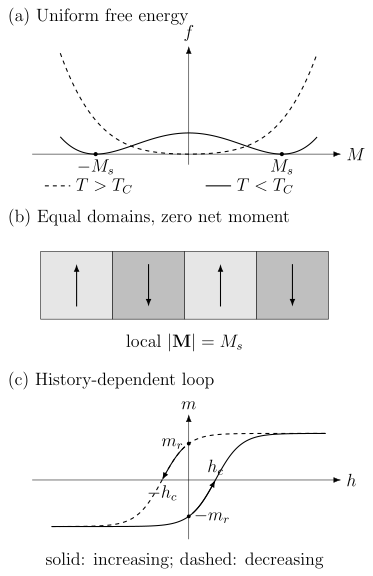
Three different descriptions of a ferromagnet: uniform free-energy minima, local order with domain cancellation, and a history-dependent response. The normalized illustrative loop uses $m_{\uparrow}=\tanh[3(h-0.35)]$ on increasing field and $m_{\downarrow}=\tanh[3(h+0.35)]$ on decreasing field, with $m=M/M_{\mathrm{sat}}$ and $h=H_{\mathrm{appl}}/H_0$ in this panel only. The upper branch is followed as the field decreases. This loop has positive energy loss; it is not an equilibrium equation of state.

Curie–Weiss Regime and Molecular Field

For localized moments of spin $S$ and number density $n$, the high-temperature Curie constant is

$$C = \frac{ \mu_0n (g\mu_{\mathrm B})^2 S(S+1) }{ 3k_{\mathrm B} }.$$

A molecular-field treatment gives

$$\chi = \frac{C}{ T-\Theta_{\mathrm{CW}} }.$$

The Weiss temperature $\Theta_{\mathrm{CW}}$ is obtained by extrapolating the high-temperature inverse susceptibility. It is not automatically the measured transition temperature.

For the exchange convention

$$H_{\mathrm{ex}} = \sum_{i<j} J_{ij} \mathbf s_i\cdot\mathbf s_j,$$

uniform local-moment mean field predicts

$$k_{\mathrm B}T_C^{\mathrm{MF}} = - \frac{ S(S+1) }{3} \sum_j J_{ij}.$$

A net ferromagnetic exchange sum makes the right-hand side positive. The same approximation gives $\Theta_{\mathrm{CW}}=T_C^{\mathrm{MF}}$.

Real fluctuations lower or reshape the transition, and competing interactions can make $\Theta_{\mathrm{CW}}$ a poor estimate of $T_C$. Curie–Weiss susceptibility is evidence for correlated magnetic degrees of freedom, not by itself proof that rigid local moments exist or that the eventual ordered state is ferromagnetic.

Domains

A uniformly magnetized finite body produces stray magnetic field outside itself. The field energy can be extensive:

$$E_{\mathrm d} = \frac{\mu_0}{2} \int_{\mathrm{all\ space}} d^3r\, |\mathbf H_{\mathrm d}|^2.$$

The sample can reduce this magnetostatic energy by forming regions with different magnetization directions. Creating more domains costs wall energy, so the equilibrium pattern balances:

• exchange stiffness, which penalizes rapid spatial rotation;
• magnetic anisotropy, which penalizes departure from easy directions;
• magnetostatic energy, which favors flux closure;
• Zeeman energy in an applied field;
• magnetoelastic energy, surfaces, and defects.

A simple micromagnetic functional for a unit direction field $\mathbf m(\mathbf r)$ is

$$F[\mathbf m] ={} \int_V d^3r \left[ A|\boldsymbol\nabla\mathbf m|^2 + K_u(1-m_z^2) - \mu_0M_s \mathbf H_{\mathrm{appl}}\cdot\mathbf m \right] + \frac{\mu_0}{2} \int_{\mathrm{all\ space}} d^3r\, |\mathbf H_{\mathrm d}|^2.$$

Here $A$ is exchange stiffness in $\mathrm{J/m}$ and $K_u>0$ an easy-axis anisotropy density in $\mathrm{J/m^3}$. Kittel and the text by Hubert and Schäfer explain the competition between wall and magnetostatic energies.

A 180-degree domain wall

For a one-dimensional wall with

$$\mathbf m = \left( 0, \sin\theta, \cos\theta \right),$$

the rotation is transverse to the wall normal $x$. Neglecting dipolar, chiral, and surface corrections, the exchange-plus-anisotropy energy per area is

$$\frac{F_{\mathrm w}}{\mathcal A} = \int dx \left[ A \left( \frac{d\theta}{dx} \right)^2 + K_u\sin^2\theta \right].$$

Minimizing this wall energy gives the ideal profile

$$\theta(x) = 2 \arctan \exp \left( \frac{x-x_0}{\Delta} \right), \qquad \Delta = \sqrt{\frac{A}{K_u}}.$$

Its wall energy is

$$\sigma_{\mathrm w} = 4\sqrt{AK_u}.$$

A commonly quoted conventional wall width is

$$\delta \simeq \pi\Delta.$$

The numerical width depends on definition and on whether the wall is Bloch-like, Néel-like, chiral, confined, or magnetostatically distorted.

For example, $A=12\,\mathrm{pJ/m}$ and $K_u=50\,\mathrm{kJ/m^3}$ give $\Delta=15.5\,\mathrm{nm}$, $\delta\simeq48.7\,\mathrm{nm}$, and $\sigma_{\mathrm w}=3.10\,\mathrm{mJ/m^2}$. Increasing anisotropy narrows the wall because it becomes more expensive to keep spins away from the easy axis; increasing exchange broadens it because rapid rotation becomes more expensive.

Demagnetizing field and sample shape

For a uniformly magnetized ellipsoid along a principal axis,

$$H_{\mathrm{int}} = H_{\mathrm{appl}} - N_dM,$$

where $N_d$ is the demagnetizing factor for that axis. The factors along three principal axes sum to one in this SI convention.

Raw susceptibility, apparent saturation field, and hysteresis shape can depend strongly on geometry. A claimed intrinsic $M(H)$ curve should state whether and how the demagnetizing correction was made.

Hysteresis and magnetic energy loss

The familiar loop $M(H)$ occurs because the system does not instantaneously find the global equilibrium minimum as field changes. Domain walls pin at defects, new domains nucleate across barriers, and coherent or incoherent rotation can remain metastable.

Key loop quantities are:

• remanent magnetization $M_r$: the moment remaining after a saturating field is removed along a specified history;
• coercive field $H_c$: the reverse field at which the measured net magnetization crosses zero;
• saturation field: an operational field range in which domain and canting changes become negligible;
• loop area: the magnetic work lost per cycle, with the appropriate SI factor and sample-volume normalization.

For a closed quasistatic cycle of a uniformly driven sample, the magnetic loss per volume is

$$\frac{W_{\mathrm{loss}}}{V} =\mu_0\oint H_{\mathrm{appl}}\,dM =-\mu_0\oint M\,dH_{\mathrm{appl}}>0$$

for the usual passive loop orientation. The unsigned geometric area in an $M$-versus-$H$ plot must therefore be multiplied by $\mu_0$ to obtain $\mathrm{J/m^3}$. Demagnetizing energy returns to its initial value after a complete cycle; rate-dependent electrical losses require additional care.

These are rate-, temperature-, geometry-, and microstructure-dependent. A soft ferromagnet can have tiny $H_c$ and nearly zero remanence. A blocked assembly of noninteracting nanoparticles can show hysteresis on laboratory timescales without constituting a bulk equilibrium ferromagnetic phase.

Equilibrium thermodynamics uses global free-energy minima and is reversible. A hysteresis loop maps metastability and dynamics. Confusing the two turns coercive behavior into a false phase definition.

Spin Waves and Low-Temperature Magnetization

Long-wavelength rotations of an ordered ferromagnet form spin waves. In an isotropic ferromagnet at zero field,

$$\epsilon(\mathbf q) \simeq D_{\alpha\beta} q_\alpha q_\beta.$$

For an isotropic solid,

$$\epsilon(\mathbf q) \simeq Dq^2.$$

The quadratic dispersion is a type-B Goldstone mode. Although two spin-rotation generators are broken, their commutator has a nonzero expectation value proportional to the magnetization, so the two transverse coordinates form one canonical pair and one magnon branch.

Magnetic anisotropy, field, dipolar coupling, finite size, or nonconservation of spin can gap or reshape the long-wavelength mode. Goldstone Modes in Many-Body Systems explains the counting, while Magnons gives the Holstein–Primakoff derivation.

Each simple ferromagnetic magnon lowers the conserved axial spin by one unit. For a three-dimensional gapless quadratic band, the thermal magnon density scales as

$$\int \frac{d^3q}{(2\pi)^3} \frac{1}{ \exp(Dq^2/k_{\mathrm B}T)-1 } \propto T^{3/2}.$$

This produces Bloch’s low-temperature law,

$$M_s(T) = M_s(0) - B_{\mathrm{Bloch}}T^{3/2} + \cdots,$$

within its regime of validity. A gap gives activated behavior at sufficiently low temperature; itinerant particle–hole excitations and magnon interactions add corrections.

Dimensionality and the Curie Temperature

The Mermin–Wagner theorem excludes nonzero-temperature ferromagnetic long-range order in one- or two-dimensional isotropic Heisenberg models with sufficiently short-range exchange. The low-energy quadratic magnons make the thermal spin-deviation integral infrared divergent in $d\le2$.

Real thin magnets can escape those assumptions through easy-axis or discrete anisotropy, sufficiently long-range dipolar interactions, or interlayer coupling that makes the system quasi-two-dimensional. A substrate or strain can matter by changing symmetry or interactions. These scales may be small compared with microscopic exchange yet decisive for the ordering temperature.

Finite lateral size has a different effect: it cuts off the longest wavelengths and can make a sample appear strongly aligned over the measurement time. It does not establish nonzero thermodynamic magnetization in the infinite short-range isotropic two-dimensional model. Finite-size rounding and slow reversal must be separated from a bulk phase transition.

Localized-Moment Ferromagnetism

In a localized-moment description, atomic or molecular moments exist over times long compared with the collective spin dynamics. Their magnitudes remain approximately fixed while exchange organizes their orientations:

$$H_{\mathrm{spin}} = \sum_{i<j} J_{ij} \mathbf s_i\cdot\mathbf s_j + H_{\mathrm{aniso}} + H_{\mathrm{dip}}.$$

A Curie–Weiss response, a recognizable atomic moment, persistent local spectral weight above $T_C$, and an appropriate magnetic entropy can support this picture together. None alone proves it: crystal fields, covalency, Kondo screening, and orbital-selective correlations alter the apparent moment.

The phrase “localized” concerns the magnetic degree of freedom, not necessarily the entire material. A local-moment ferromagnet can coexist with conduction electrons that mediate RKKY exchange or carry spin-polarized current.

Itinerant Ferromagnetism

In an itinerant ferromagnet, the same delocalized electrons form bands and develop a spin-polarized occupation. The canonical Stoner Criterion derivation compares the band-energy cost of transferring particles between spin-resolved Fermi seas with the exchange-energy gain.

For a paramagnetic density of states per spin $N(E_{\mathrm F})$ and a matching scalar interaction $I$, the uniform unpolarized state loses quadratic mean-field stability when

$$I\,N(E_{\mathrm F}) >1.$$

The threshold explains why a large density of states can promote ferromagnetism, but it does not determine the ordered moment or Curie temperature. The scalar Stoner model neglects finite-wavevector competitors, strong dynamical spin fluctuations, nonlocal correlations, detailed orbital structure, and the possibility that sizable local moments survive above $T_C$. It is a starting point for the material discussion, not a complete theory of metallic magnets.

A continuum, not a binary classification

Local-moment and itinerant language describe limiting organizations:

Question	Local-moment limit	Itinerant limit
What orders?	Pre-existing moment orientations	Spin polarization of bands
Above $T_C$	Moment amplitude can persist	Polarization may collapse
Natural model	Spin Hamiltonian	Interacting band model
Low-energy charge	Can be gapped	Usually metallic
Primary scale	Exchange among moments	Bandwidth, density of states, interaction

Real iron, cobalt, nickel, rare-earth metals, and correlated ferromagnets need not sit at either endpoint. Hund coupling can create robust local moments in a metal, while itinerant carriers determine their coherence and exchange. A trustworthy analysis asks which moment amplitudes, time scales, orbitals, and wavevectors are actually resolved.

Recognizing ferromagnetic order in measurements

Magnetic Susceptibility explains background and geometry corrections for $M(H,T)$. Extrapolating a high-field branch to zero internal field can estimate $M_s$, provided unsaturated components are modeled. Near $T_C$, compare this estimate with susceptibility, heat capacity, or critical scattering. A straight Arrott plot follows a chosen equation of state; it does not prove mean-field exponents.

Magnetic diffraction determines the ordered structure. Uniform magnetic intensity can overlap nuclear Bragg peaks, so polarization analysis or temperature dependence helps separate them. Domain imaging explains spatial cancellation, while local probes distinguish static order from slow or fast fluctuations. Magnetic contrast must be separated from topographic or strain contrast.

Finally, compare the excitations and electronic state. A local-moment model should reproduce static order and dynamic spectral weight; an itinerant model should account for band polarization and collective modes. Spin Waves and Magnons in Materials connects exchange models to measured dispersion and intensity.

Distinguishing Nearby Magnetic States

State	Uniform moment	Internal pattern	Defining distinction
Ferromagnet	Nonzero in a selected domain	Equivalent moments align uniformly	Primary order is $\mathbf Q=0$ magnetization
Ferrimagnet	Usually nonzero	Opposing unequal sublattices	Net moment is a difference of sublattice orders
Canted antiferromagnet	Small nonzero component possible	Primary staggered order	Uniform moment is secondary to Néel order
Spin glass	Sample-dependent frozen moment	Random, nonperiodic freezing	No conventional uniform long-range order
Superparamagnet	Time-window dependent	Finite ferromagnetic particles fluctuate	Blocking is not a bulk equilibrium transition
Paramagnet	Zero at zero field	No spontaneous uniform order	Magnetization is induced and vanishes with field

A nonzero net moment does not alone identify ferromagnetism. The ordering wavevector, sublattice structure, thermodynamic limit, and time dependence decide the classification.

Exercises

1. Why the thermodynamic limit comes first

Suppose a finite easy-axis magnet has an exact symmetry that sends $M\to-M$. Explain why its zero-field Gibbs state has $\langle M\rangle=0$, and why this does not exclude ferromagnetism.

Solution

Let $U$ implement the symmetry. Since $[U,H]=0$ and $UMU^\dagger=-M$, the finite-volume Gibbs operator $\rho=e^{-\beta H}/Z$ commutes with $U$. Then

$$\langle M\rangle = \operatorname{Tr}(\rho M) = \operatorname{Tr} \left( \rho UMU^\dagger \right) = -\langle M\rangle,$$

so $\langle M\rangle=0$. Ferromagnetism concerns the infinite-volume family. Taking $V\to\infty$ in a small selecting field can produce one extremal state, after which the field may be removed while a nonzero magnetization remains.

2. Landau minima and susceptibility

For

$$f(M) = \frac{a_0}{2}(T-T_C)M^2 + \frac{b}{4}M^4 - hM,$$

derive the zero-field minima and the susceptibility above and below $T_C$.

Solution

At $h=0$,

$$\frac{\partial f}{\partial M} = M \left[ a_0(T-T_C)+bM^2 \right] = 0.$$

For $T>T_C$, the stable solution is $M=0$. For $T<T_C$,

$$M_s^2 = \frac{a_0(T_C-T)}{b}.$$

Differentiate the equation of state

$$h = a_0(T-T_C)M+bM^3.$$

Above $T_C$,

$$\chi_h^+ = \frac{1}{a_0(T-T_C)}.$$

Below $T_C$, evaluate the derivative at $M=M_s$:

$$\chi_h^- = \frac{1}{ a_0(T-T_C)+3bM_s^2 } = \frac{1}{ 2a_0(T_C-T) }.$$

3. Mean-field Curie temperature

A nearest-neighbor spin-$1/2$ model has coordination $z=6$ and $J=-4\,\mathrm{meV}$ in the convention $H=J\sum_{\langle i,j\rangle}\mathbf s_i\cdot\mathbf s_j$. Estimate $T_C^{\mathrm{MF}}$.

Solution

The exchange sum is

$$\sum_jJ_{ij} = zJ = -24\,\mathrm{meV}.$$

For $S=1/2$, $S(S+1)=3/4$, so

$$k_{\mathrm B}T_C^{\mathrm{MF}} = - \frac{3/4}{3} \left( -24\,\mathrm{meV} \right) = 6\,\mathrm{meV}.$$

Using $k_{\mathrm B}=0.08617\,\mathrm{meV/K}$ gives

$$T_C^{\mathrm{MF}} \simeq 69.6\,\mathrm K.$$

This is a convention-specific mean-field estimate, not a prediction that includes critical fluctuations.

4. What can a wall measurement determine?

A wall-profile fit gives $\Delta=15\,\mathrm{nm}$, and an independent measurement gives $\sigma_{\mathrm w}=3.2\,\mathrm{mJ/m^2}$. Assume the exchange-plus-uniaxial model above, with negligible dipolar, chiral, and surface corrections. Determine $A$ and $K_u$. Would the width alone suffice, and what changes if an unknown Dzyaloshinskii–Moriya coupling lowers the wall energy?

Solution

The two measurements constrain different combinations:

$$\Delta^2=\frac{A}{K_u},\qquad \sigma_{\mathrm w}=4\sqrt{AK_u}.$$

Multiplying and dividing give

$$A=\frac{\sigma_{\mathrm w}\Delta}{4} =12\,\mathrm{pJ/m},\qquad K_u=\frac{\sigma_{\mathrm w}}{4\Delta} \simeq53.3\,\mathrm{kJ/m^3}.$$

The measured profile parameter is $\Delta$, not the conventional width $\delta=\pi\Delta$. Substituting $\delta$ would overestimate $A$ by $\pi$ and underestimate $K_u$ by the same factor. A width alone fixes only the ratio $A/K_u$: scaling both coefficients by any positive factor leaves the profile unchanged.

For the ideal chiral wall, Magnetic Anisotropy gives $\sigma_{\mathrm w}=4\sqrt{AK_u}-\pi|D|$, while the width remains $\sqrt{A/K_u}$. If $D$ is unknown, even these two measurements leave a family of possible $A,K_u,D$. The values above are therefore model-dependent inferences, not direct readings of two intrinsic constants.

5. Bloch-law scaling

Use $\epsilon(\mathbf q)=Dq^2$ to show by rescaling momentum that the thermal magnon density in three dimensions is proportional to $T^{3/2}$.

Solution

The density is

$$n_m = \int \frac{d^3q}{(2\pi)^3} \frac{1}{ e^{Dq^2/k_{\mathrm B}T}-1 }.$$

Set

$$\mathbf q = \sqrt{\frac{k_{\mathrm B}T}{D}} \mathbf x.$$

Then $d^3q=(k_{\mathrm B}T/D)^{3/2}d^3x$, while the Bose factor becomes $1/(e^{x^2}-1)$. The remaining dimensionless integral is temperature independent, so

$$n_m \propto \left( \frac{k_{\mathrm B}T}{D} \right)^{3/2}.$$

Each magnon reduces the axial magnetization, yielding the leading $T^{3/2}$ law.

To explore departures from uniform order, continue to Antiferromagnetism and Ferrimagnetism. 2D Magnets and Ferroelectrics treats thin-layer systems, and Skyrmions and Magnetic Textures develops nonuniform magnetization patterns.

References

• A. Aharoni, Introduction to the Theory of Ferromagnetism, 2nd ed. (Oxford University Press, 2001), doi:10.1093/oso/9780198508083.001.0001.
• F. Bloch, “Zur Theorie des Ferromagnetismus,” Zeitschrift für Physik 61, 206–219 (1930), doi:10.1007/BF01339661.
• J. M. D. Coey, Magnetism and Magnetic Materials (Cambridge University Press, 2010), doi:10.1017/CBO9780511845000.
• A. Hubert and R. Schäfer, Magnetic Domains: The Analysis of Magnetic Microstructures (Springer, 1998), doi:10.1007/978-3-540-85054-0.
• C. Kittel, “Theory of the Structure of Ferromagnetic Domains in Films and Small Particles,” Physical Review 70, 965–971 (1946), doi:10.1103/PhysRev.70.965.
• N. D. Mermin and H. Wagner, “Absence of Ferromagnetism or Antiferromagnetism in One- or Two-Dimensional Isotropic Heisenberg Models,” Physical Review Letters 17, 1133–1136 (1966), doi:10.1103/PhysRevLett.17.1133.