Ferrimagnetism

Ferrimagnetism is ordered magnetism with inequivalent opposing sublattices whose moments generally do not cancel. Their imbalance produces a uniform magnetic moment, while their antiparallel coupling supports exchange-driven collective motion. A ferrimagnet can also pass through a temperature at which the moments cancel without losing its internal order. Understanding that compensation requires keeping magnetic moment, angular momentum, and domain averaging distinct.

Required background. Magnetic Moments in Matter relates magnetic moments to spin and orbital angular momentum. Ferromagnetism introduces domains, and Antiferromagnetism introduces opposing sublattices and their ordering patterns.

Helpful background. Exchange Interactions explains the microscopic couplings that favor antiparallel alignment.

Unequal Opposing Sublattices

Here $\mathbf M_A$ and $\mathbf M_B$ are the contributions of the two sublattices per total sample volume, in amperes per metre. Their sum is the physical bulk magnetization. For a collinear domain, write

$$\mathbf M_A=M_A\mathbf n,\qquad \mathbf M_B=-M_B\mathbf n,\qquad M_A,M_B>0.$$

Then

$$\begin{aligned} \mathbf M&=\mathbf M_A+\mathbf M_B=(M_A-M_B)\mathbf n,\\ \mathbf L&=\mathbf M_A-\mathbf M_B=(M_A+M_B)\mathbf n. \end{aligned}$$

$\mathbf M$ measures the imbalance; $\mathbf L$ measures the antiparallel order. A half-sum convention is also common, but its sublattice inputs must be normalized consistently before comparing a calculated quantity with measured magnetization. Unequal site populations belong inside $M_A$ and $M_B$, not in an extra factor inserted afterward.

Why a uniform moment is allowed

Consider order at zero propagation vector relative to the chemical lattice, with $A$ and $B$ already present in the chemical basis. If a symmetry interchanges equivalent sublattices, it sends $\mathbf L\to-\mathbf L$ while leaving $\mathbf M$ unchanged. It therefore forbids a free-energy term $\mathbf M\cdot\mathbf L$.

For inequivalent sublattices, that interchange need not be a symmetry. A permitted free-energy density can contain

$$f=\frac{r_M}{2}M^2+\frac{r_L}{2}L^2 +\lambda\mathbf M\cdot\mathbf L+\cdots.$$

For $r_M>0$, minimization gives $\mathbf M=-\lambda\mathbf L/r_M+\cdots$: uniform magnetization accompanies the antiparallel order. The zero-wavevector assumption matters. Translation symmetry forbids a bilinear coupling between uniform $\mathbf M_0$ and an order parameter $\mathbf L_{\mathbf Q}$ at a nonzero chemical wavevector, even if some sites are inequivalent.

Spin Counting and the Quantum Ground State

A minimal localized model has dimensionless spins and antiferromagnetic coupling,

$$H=\sum_{\langle i\in A,j\in B\rangle}J_{ij}\mathbf S_i\cdot\mathbf s_j, \qquad J_{ij}>0.$$

For a collinear cell with $n_A$ spins of length $S_A$ and $n_B$ of length $S_B$, the classical spin imbalance is $\lvert n_AS_A-n_BS_B\rvert$. With quenched orbital moments and scalar $g$ factors, the corresponding ionic estimate is

$$\mu_{\mathrm{cell}}\simeq\mu_{\mathrm B} \left|n_Ag_AS_A-n_Bg_BS_B\right|.$$

This is a saturated moment estimate, using $gS$, not the paramagnetic effective moment $g\sqrt{S(S+1)}$. Covalency, orbital contributions, canting, and quantum fluctuations can change measured sublattice moments.

There is also an exact finite-system result. For a connected bipartite isotropic Heisenberg model with positive intersublattice exchanges and no same-sublattice exchange, the Lieb–Mattis theorem gives

$$S_{\mathrm{ground}}= \left|\sum_{i\in A}S_i-\sum_{j\in B}S_j\right|.$$

The unequal sums produce a ground-state spin multiplet. This theorem does not identify each local moment with its fully polarized value, and a finite-system multiplet alone does not establish a finite-temperature ordered phase. Frustration, anisotropy, and itinerant charge fluctuations require separate analysis (Lieb and Mattis, 1962).

Sublattice Thermal Curves and the Curie Temperature

Different exchange fields, spin lengths, crystal-field levels, and magnon populations can make the ratio $M_A(T)/M_B(T)$ vary with temperature. In a three-dimensional ferrimagnet with one continuous ordering transition, both sublattices vanish at a common Curie temperature $T_C$. When they couple to the same critical mode with nonzero amplitudes, they share its leading critical exponent; different temperature dependences do not imply different asymptotic exponents.

A simple molecular-field example makes the coupled instability explicit. Above the transition, let $m_A,m_B$ be signed contributions along a uniform source $h$, and take only an antiferromagnetic intersublattice coefficient $\lambda>0$:

$$m_A=\frac{C_A}{T}(h-\lambda m_B),\qquad m_B=\frac{C_B}{T}(h-\lambda m_A).$$

Here the Zeeman energy density is $-h(m_A+m_B)$, so $h$ is in tesla, $C_\alpha$ in $\mathrm{A\,K/(m\,T)}$, and $\lambda$ in $\mathrm{T\,m/A}$. Solving the two linear equations gives

$$T_C^{\mathrm{MF}}=\lambda\sqrt{C_AC_B},\qquad \chi_h=\frac{\partial(m_A+m_B)}{\partial h} =\frac{T(C_A+C_B)-2\lambda C_AC_B} {T^2-\lambda^2C_AC_B}.$$

Thus inverse susceptibility need not be a straight Curie–Weiss line. When $C_A=C_B=C$, the uniform response simplifies to $2C/(T+\lambda C)$: it stays finite at the staggered instability. Unequal constants generally let the critical mode carry a uniform moment. Intrinsic susceptibility with respect to $H$ is $\chi_H=\mu_0\chi_h$.

This mean-field example neglects fluctuations. An isolated one-dimensional model with short-range interactions does not acquire finite-temperature long-range order merely by adding easy-axis anisotropy; even the short-range Ising chain has no positive-temperature transition. Interchain coupling or sufficiently long-range interactions can change that conclusion. Slow finite-sample reversal is also different from thermodynamic order.

Magnetization Compensation

A magnetization compensation temperature $T_M<T_C$ satisfies

$$M_A(T_M)=M_B(T_M)=M_0>0.$$

Consequently $\mathbf M=0$, but $\mathbf L=2M_0\mathbf n$ remains nonzero. No symmetry need be restored and the free energy need not be singular. Compensation is usually a zero of one observable inside an ordered phase.

Across $T_M$, the dominant sublattice changes. In a pinned domain, the signed magnetization reverses relative to the tracked $A$ direction. In an equilibrated weak field, the entire domain can reverse instead. A magnetometer therefore need not display a signed crossing unless the domain orientation and measurement protocol are controlled.

For a transparent illustrative model, set $t=T/T_C$ and

$$M_A=M_{A0}\sqrt{1-t}(1-ct),\qquad M_B=M_{B0}\sqrt{1-t},\qquad 0<c<1.$$

Both curves share the same leading critical power. Their ratio still changes, allowing compensation when

$$\frac{T_M}{T_C}=\frac{1-r}{c}\in(0,1), \qquad r=\frac{M_{B0}}{M_{A0}}.$$

These are illustrative curves, not a fit or a universal temperature law. Some ferrimagnets have no compensation point.

Angular-Momentum Compensation

Magnetic moment and angular momentum need not cancel together. Assume rigid collinear sublattice moments with electronlike gyromagnetic signs, $\boldsymbol\mu_\alpha=-\gamma_\alpha\mathbf J_\alpha$, where $\gamma_\alpha>0$ is a magnitude. The physical angular-momentum density is then

$$\mathbf j_{\mathrm{net}}= -\left(\frac{M_A}{\gamma_A}-\frac{M_B}{\gamma_B}\right)\mathbf n.$$

Its compensation temperature $T_A<T_C$ satisfies

$$\frac{M_A(T_A)}{\gamma_A}=\frac{M_B(T_A)}{\gamma_B}.$$

If the gyromagnetic ratios are equal, existing compensation points coincide. Otherwise $T_A$ and $T_M$ generally differ, and either may be absent. With $\gamma_\alpha=g_\alpha\mu_{\mathrm B}/\hbar$, the model above gives

$$\frac{T_A}{T_C}=\frac{1-rg_A/g_B}{c},$$

provided this value lies strictly between zero and one. For $M_{A0}=1.2$, $M_{B0}=1$, $c=0.5$, $g_A=2$, and $g_B=1.8$, the two temperatures are $T_M/T_C=1/3$ and $T_A/T_C=4/27$.

In an isotropic spin model, the expectation of the commutator of broken rotation generators is proportional to net angular momentum. A nonzero value leads to ferromagnetic-like, quadratic low-energy motion. Cancellation can suppress the first-order gyrotropic term and reveal antiferromagnetic-like inertial dynamics. Actual crystals also have spin–orbit coupling, anisotropy, damping, and coupling to the lattice, so this is not a general claim of exact gapless modes at $T_A$. The assumed moment-to-angular-momentum conversion must itself be appropriate to the material. Kim et al. (2017) demonstrate the distinction through enhanced domain-wall motion near angular-momentum compensation.

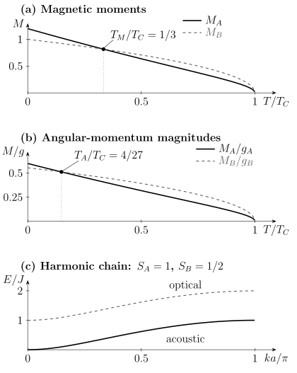
Top and middle: the illustrative thermal curves defined above cross at $T_M/T_C=1/3$ and $T_A/T_C=4/27$. Both sublattices remain ordered at either crossing. Bottom: a separate zero-temperature alternating-spin-chain calculation with $S_A=1$ and $S_B=1/2$. The curves are linear-spin-wave energies, not exact excitation energies of an arbitrary ferrite.

Collective Modes

Two coupled sublattices support an acoustic motion in which the common axis changes slowly while the moments remain nearly antiparallel, and an optical motion that strongly changes their relative angle. “Optical” does not imply that light couples efficiently to the mode. A ferrite with many spins per primitive cell has many branches.

Alternating-spin-chain benchmark

Take a cell of length $a$, spins $S_A>S_B$, and bonds $A_n$–$B_n$ and $B_n$–$A_{n+1}$, each with $J>0$. At zero temperature, linear spin-wave theory about the collinear state gives, with $\Delta S=S_A-S_B$,

$$E_\pm(k)=\hbar\omega_\pm(k) =J\left[\sqrt{(\Delta S)^2+4S_AS_B\sin^2(ka/2)} \ \pm\Delta S\right].$$

The lower branch has $E_-(0)=0$ and the upper branch has $E_+(0)=2J\Delta S$. Expanding the square root gives

$$E_-(k)\simeq\frac{JS_AS_B}{2\Delta S}(ka)^2, \qquad |ka|\sqrt{S_AS_B}\ll\Delta S.$$

The condition matters: this quadratic expansion is not uniform as $\Delta S\to0$. Taking equal spins in the full harmonic formula gives linear branches, but it does not prove Néel order in an equal-spin one-dimensional quantum chain. Its exact physics depends on spin and interactions.

For $S_A=1,S_B=1/2$, the harmonic optical gap is $J$, and the zone-edge energies are $J$ and $2J$. Quantum corrections shift the optical branch; numerical work by Yamamoto, Brehmer, and Mikeska (1998) distinguishes the robust gapless/gapped pattern from harmonic numerical predictions. General quantization is developed in Magnons, and material spectra in Spin Waves and Magnons.

The two branches can carry opposite spin changes. Their unequal thermal populations help explain different sublattice thermal curves. In a multi-branch, anisotropic material, mode mixing makes a single assigned spin per magnon inadequate without specifying the mode and wavevector.

Ferrites and Other Material Realizations

Ferrites are iron-containing oxides with magnetic ions on several crystallographic sites. Many are ferrimagnetic insulators, with oxygen-mediated superexchange opposing important sublattice moments. Site occupancy, valence, and canting matter as much as the chemical label.

In ideal inverse-spinel magnetite,

$$(\mathrm{Fe}^{3+})_A[\mathrm{Fe}^{3+}\mathrm{Fe}^{2+}]_B\mathrm O_4,$$

the high-spin, spin-only saturated moments are approximately $5\mu_{\mathrm B}$ for $\mathrm{Fe}^{3+}$ and $4\mu_{\mathrm B}$ for $\mathrm{Fe}^{2+}$. Opposing trivalent moments cancel, leaving $4\mu_{\mathrm B}$ per formula unit in this ionic picture. Mixed valence, covalency, and the low-temperature Verwey transition require more than this count.

In yttrium iron garnet, $\mathrm Y_3\mathrm{Fe}_5\mathrm O_{12}$, nonmagnetic yttrium accompanies two opposing groups of two and three trivalent iron ions per formula unit. The ideal imbalance is therefore $5\mu_{\mathrm B}$ per formula unit. Its large magnetic basis produces many magnon branches; a single effective moment describes only a restricted long-wavelength range (Cherepanov et al., 1993). Magnetic rare-earth substitution adds another sublattice and can introduce compensation or reorientation.

Rare-earth–transition-metal alloys such as GdFeCo provide distinct magnetic and angular-momentum compensation scales. A synthetic ferrimagnet instead consists of antiferromagnetically coupled ferromagnetic layers with unequal areal moments: layer thickness is part of the moment count. Alternating-spin molecules and chains offer finite-system and low-dimensional realizations, with the thermal limitations discussed above.

Material uses follow physical compromises. High resistivity suppresses eddy-current loss in soft ferrites, while strong anisotropy favors coercivity in hard ferrites. Low damping is valuable for propagating spin waves, but propagation also depends on mode velocity, interfaces, and disorder. Compensation can reduce dipolar fields or alter texture motion; it does not by itself guarantee faster switching or lower dissipation. See Spintronics for transport and torque mechanisms.

Domains, Compensation, and Measurements

Away from compensation, the net moment creates dipolar fields and can form flux-reducing domains. Remanence, coercivity, and loop losses then depend on pinning, geometry, and sweep rate as well as intrinsic exchange. The SI loss density is $\mu_0\oint H_{\mathrm{appl}}\,dM$; its origin and sign are explained in Ferromagnetism. Near $T_M$, the Zeeman coupling to the small net moment weakens while anisotropy can remain substantial. Large coercivity is possible, but a universal divergence is not implied.

Bulk magnetometry alone measures a spatial average. To distinguish intrinsic compensation from equal populations of opposite domains, combine it with a controlled field/temperature protocol, domain imaging, and sublattice-sensitive measurements. Neutron diffraction can determine magnetic site patterns, while element-selective x-ray magnetic dichroism can separate contributions from different species. Separate sites of the same element may require additional structural or spectroscopic modeling. Signals must be converted into comparably normalized moments before declaring a crossing.

Resonance frequencies and field slopes constrain effective gyromagnetic ratios and exchange-coupled modes; a static magnetization zero alone does not locate $T_A$. Likewise, an anomalous Hall signal weights electronic states and scattering, so its zero need not coincide with either compensation temperature. A finite applied field can cant the sublattices and induce a nonzero magnetization even at the zero-field $T_M$.

Observation	What it establishes	What remains to distinguish
Unequal opposing ordered sublattice moments	Ferrimagnetic order in the measured state	Domain average and moment normalization
Vanishing bulk low-field moment	A small spatially averaged magnetization	Intrinsic compensation, domains, or loss of order
Equal opposing sublattice moment densities below $T_C$	Magnetization compensation	Angular momentum still depends on gyromagnetic ratios
Exchange-coupled dynamics with compensated angular momentum	An angular-momentum compensation regime under the fitted model	Anisotropy, damping, and lattice coupling

Exercises

1. Two compensation temperatures

Use the illustrated curves with $M_{A0}=1.2$, $M_{B0}=1$, $c=0.5$, $g_A=2$, and $g_B=1.8$. Find $T_M/T_C$ and $T_A/T_C$, and determine which quantity remains nonzero at each.

Solution

Cancel the common positive factor $\sqrt{1-t}$ for $t<1$. Moment compensation requires $1.2(1-t/2)=1$, giving $t_M=1/3$. Angular-momentum compensation requires $1.2(1-t/2)/2=1/1.8$, giving $t_A=4/27$.

At $t_M$, the signed angular-momentum difference in units with the common $\hbar/\mu_{\mathrm B}$ omitted is

$$\frac{M_A}{g_A}-\frac{M_B}{g_B} =\sqrt{2/3}\left(\frac12-\frac1{1.8}\right)\ne0.$$

The physical angular momentum has the opposite sign along $\mathbf n$. At $t_A$, $M_A/M_B=g_A/g_B=10/9$, so $M_A-M_B=M_B/9>0$. The point $t=1$, where both moments vanish, is the ordering transition and is excluded from either compensation condition.

2. The crossover from quadratic to linear waves

Derive the small-$k$ acoustic energy and its range of validity. Evaluate both branch energies at $k=0$ and $k=\pi/a$ for $S_A=1,S_B=1/2$. Why can the small-$k$ expansion not be used to set $S_A=S_B$?

Solution

Using $\sin(ka/2)\simeq ka/2$, expand

$$\sqrt{(\Delta S)^2+S_AS_B(ka)^2} =\Delta S+\frac{S_AS_B(ka)^2}{2\Delta S}+\cdots.$$

This requires $S_AS_B(ka)^2\ll(\Delta S)^2$. The acoustic coefficient follows after subtracting $\Delta S$. The requested pairs $(E_-,E_+)$ are $(0,J)$ and $(J,2J)$.

The allowed quadratic region shrinks to zero as $\Delta S\to0$. Instead use the full expression at $S_A=S_B=S$, obtaining $E_\pm=2JS\lvert\sin(ka/2)\rvert\simeq JS\lvert ka\rvert$. These remain harmonic predictions, not a proof of the equal-spin chain’s ground-state order.

3. A finite unequal-spin pair

For $H=J\mathbf S\cdot\mathbf s$ with $S=1$, $s=1/2$, and $J>0$, find the ground-state total spin and the excitation gap. Does this one bond have the same optical gap as the harmonic chain?

Solution

Angular-momentum addition gives total spins $F=1/2,3/2$ and

$$E_F=\frac J2\left[F(F+1)-S(S+1)-s(s+1)\right].$$

The energies are $-J$ and $J/2$, so the ground state is a doublet and the gap is $3J/2$. The ground spin agrees with $|S-s|$. Its gap differs from the chain’s harmonic value $J$: the graph, coordination, and approximation differ. A spin-counting theorem fixes the ground multiplet, not every excitation energy.

4. A zero magnetometer signal

A low-field magnetization crosses zero, imaging shows equal opposite domains, and calibrated element-resolved moments remain unequal. A high-field measurement is positive. Is intrinsic compensation established?

Solution

No. Equal domains already explain the bulk zero, while unequal opposing sublattice moment densities rule out compensation under the assumed two-sublattice interpretation. The high-field result alone would not suffice: even a compensated state can develop an induced moment by canting. Track a selected domain and compare the correctly normalized sublattice moments, using sufficiently weak fields or a justified zero-field extrapolation.

References

• V. Cherepanov, I. Kolokolov, and V. L’vov, “The Saga of YIG: Spectra, Thermodynamics, Interaction and Relaxation of Magnons in a Complex Magnet,” Physics Reports 229, 81–144 (1993), doi:10.1016/0370-1573(93)90107-O.
• J. M. D. Coey, Magnetism and Magnetic Materials (Cambridge University Press, 2010), doi:10.1017/CBO9780511845000.
• K.-J. Kim et al., “Fast Domain Wall Motion in the Vicinity of the Angular Momentum Compensation Temperature of Ferrimagnets,” Nature Materials 16, 1187–1192 (2017), doi:10.1038/nmat4990.
• E. Lieb and D. Mattis, “Ordering Energy Levels of Interacting Spin Systems,” Journal of Mathematical Physics 3, 749–751 (1962), doi:10.1063/1.1724276.
• J. Smit and H. P. J. Wijn, Ferrites (Philips Technical Library, 1959).
• S. Yamamoto, S. Brehmer, and H.-J. Mikeska, “Elementary Excitations of Heisenberg Ferrimagnetic Spin Chains,” Physical Review B 57, 13610–13613 (1998), doi:10.1103/PhysRevB.57.13610.