Strange Metals

A strange metal is an experimentally identified metallic regime whose response departs from the simplest low-temperature Fermi-liquid transport laws. The term describes an observed pattern; it does not require that every useful quasiparticle description has already been excluded. The most familiar signature is an electrical resistivity proportional to temperature over an unusually broad interval, sometimes continuing to the lowest accessible normal-state temperature. The stronger cases also show anomalous optical, thermodynamic, spectroscopic, or magnetotransport behavior.

The name is operational, not a microscopic classification. Strange metals in cuprates, iron-based superconductors, organic conductors, heavy-fermion compounds, and moiré systems need not belong to one phase or universality class. Nor does every linear-$T$ resistivity imply strong electronic correlations: conventional electron–phonon scattering is approximately linear at temperatures above the Bloch–Grüneisen scale.

A trustworthy analysis therefore separates three claims:

1. Phenomenology: a stated observable has a reproducible anomalous dependence over a stated window.
2. Rate extraction: a transport or optical model converts that observable into a relaxation scale of order $k_{\mathrm B}T/\hbar$.
3. Mechanism: a theory explains the same coefficients, tuning trends, and independent probes.

Evidence for the first claim does not establish the second or third.

Required background. Drude Theory supplies the carrier, mass, and relaxation-time assumptions behind a rate extracted from resistivity. Boltzmann Transport supplies collision-weighted current relaxation. Fermi Liquid Theory Preview supplies the ordinary quasiparticle baseline, while Non-Fermi Liquids distinguishes failure of that baseline from identification of a replacement mechanism.

Strange and Bad Metals

The term bad metal usually emphasizes that resistivity exceeds a conventional saturation or mean-free-path estimate. The term strange metal emphasizes anomalous low-energy laws. A material may be both, either, or neither. The metals, insulators, and semiconductors guide develops the broader classification.

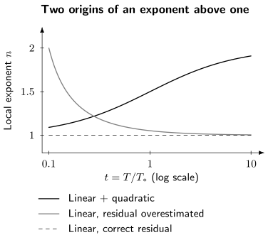
Two reasons for a local exponent above one. The rising curve is $n_{\rm eff}=(1+2t)/(1+t)$ for a mixed law, with $t=T/T_*$ and $T_*=A_1/A_2$. The falling curve is $n_{\rm app}=t/(t-0.05)$ for an exactly linear law whose residual resistivity was overestimated by $0.05AT_*$. The dashed line is the correctly subtracted linear law. These calculated examples connect to Exercises 1 and 3; they are not fits to a material.

Linear-in-Temperature Resistivity

The empirical law

The minimal low-temperature fit is

$$\rho(T) = \rho_0+A_1T,$$

where $\rho_0$ is the residual resistivity and $A_1$ is the linear coefficient. Real data often require additional terms,

$$\rho(T) = \rho_0+A_1T+A_2T^2+\rho_{\mathrm{other}}(T).$$

The terms need not represent independent scattering probabilities. Matthiessen’s rule can fail when anisotropic channels, multiple bands, hydrodynamic flow, or temperature-dependent carrier densities are present. A good polynomial fit is consequently a description of a window, not a decomposition into microscopic processes.

A useful local diagnostic is the local logarithmic exponent

$$n_{\mathrm{eff}}(T) = \frac{d\ln[\rho(T)-\rho_0]}{d\ln T} = \frac{T}{\rho(T)-\rho_0} \frac{d\rho}{dT}.$$

Differentiation amplifies noise, so the smoothing scale and its uncertainty must be shown. An extended plateau near $n_{\mathrm{eff}}=1$ is stronger evidence for linearity than the visual straightness of one plot. It also exposes sensitivity to the chosen $\rho_0$: an incorrect residual subtraction can manufacture an apparent exponent drift.

Why the low-temperature limit matters

At temperatures well above an acoustic-phonon Bloch–Grüneisen scale, the thermally occupied phonon phase space gives an approximately linear resistivity. At low temperature in a clean three-dimensional metal, the corresponding Bloch–Grüneisen contribution instead falls rapidly, commonly as $T^5$ under standard assumptions. This is why linearity extending below all identified phonon and coherence scales is the more discriminating observation.

Superconductivity or another ordered phase often hides that limit. Magnetic field, pressure, disorder, or composition can expose a normal state, but each tuning method is an intervention. A field can reconstruct or polarize the electronic state; chemical substitution can change disorder and carrier density. A responsible claim states the tuning path and tests whether the inferred slope is continuous across it.

Mean-free-path heuristics

In a simple isotropic metal one may estimate

$$\ell_{\mathrm{tr}} = v_{\mathrm F}\tau_{\mathrm{tr}}, \qquad k_{\mathrm F}\ell_{\mathrm{tr}} \sim 1$$

at the Mott–Ioffe–Regel crossover. This is a useful warning that a semiclassical wave packet is losing spatial coherence. It is not a sharp universal boundary. Multiband currents, incoherent spectral weight, anisotropic Fermi surfaces, and uncertain carrier densities make $k_{\mathrm F}\ell$ model dependent. Exceeding a heuristic saturation resistivity does not by itself identify the strange-metal mechanism.

Planckian Scattering Language

A dimensionless rate

The Planckian parametrization writes a chosen relaxation rate as

$$\frac{\hbar}{\tau_X(T)} = \alpha_X k_{\mathrm B}T,$$

where the subscript $X$ must identify the channel: dc transport, optical current relaxation, single-particle decay, energy relaxation, phase decoherence, or another process. Saying only “the lifetime” hides an essential physical choice.

The thermal time $\tau_T=\hbar/(k_{\mathrm B}T)$ is the only time scale that can be constructed from $T$, $k_{\mathrm B}$, and $\hbar$. A fitted $\alpha_X$ of order unity can therefore signal scale-free dynamics. It is not presently an established universal upper bound on all quantum relaxation rates. The energy–time uncertainty relation does not derive such a bound, and different correlation functions can relax at parametrically different rates in the same system.

From a resistivity slope to a rate

Under a one-band Drude interpretation,

$$\rho = \frac{m^*}{ne^2\tau_{\mathrm{tr}}}.$$

For temperature-independent $n/m^*$ and a separable residual rate, combining this relation with $\rho-\rho_0=A_1T$ gives

$$\alpha_{\mathrm{tr}} = \frac{\hbar ne^2}{k_{\mathrm B}m^*} A_1.$$

This conversion is informative only after $n$ and $m^*$ have been defined and measured consistently. In a correlated multiband material, the relevant quantity is a current-carrying spectral weight rather than a unique thermodynamic mass. Fermi-surface anisotropy, vertex corrections, parallel bands, and temperature-dependent coherent weight can all change the inferred $\alpha_{\mathrm{tr}}$ without changing the measured $A_1$.

One can see the ambiguity directly by defining $\mathcal D=ne^2/m^*$ and $\Gamma=1/\tau$ through $\sigma(\omega)=\mathcal D/(\Gamma-i\omega)$. Then

$$\frac{d\rho}{dT} =\frac{1}{\mathcal D}\frac{d\Gamma}{dT} -\frac{\Gamma}{\mathcal D^2}\frac{d\mathcal D}{dT}.$$

A slope can reflect changing current-carrying weight as well as a changing rate. Optical measurements help separate these possibilities; a thermodynamic mass alone need not determine $\mathcal D$.

For several independent conducting channels at zero Hall response along a principal axis,

$$\sigma_{\mathrm{dc}} = \sum_a \sigma_a, \qquad \rho_{\mathrm{dc}} = \frac{1}{\sum_a \sigma_a},$$

so resistivities cannot generally be assigned band by band and added. The longest-lived or highest-weight channel may short-circuit strongly scattered regions of the Fermi surface.

Material Families

No single material family supplies every diagnostic, and the same label hides different experimental constraints.

Family	Useful comparison and limitation
Hole-doped cuprates	Low-temperature linear resistivity and material-dependent scattering anisotropy; account for pseudogap, charge order, field and carrier-weight changes.
Iron pnictides	Linear transport near magnetic or nematic tuning; multiband compensation and intertwined order complicate the exponent.
Quasi-one-dimensional organics	Pressure connects a linear component with spin fluctuations and pairing; dimensional crossover limits extrapolation.
Heavy fermions	Thermodynamic anomalies and reconstruction can accompany linear transport; small coherence scales and magnetic fields affect the interpretation.
Moiré systems	Gate-tunable large slopes in narrow bands; phonons and angle inhomogeneity can also be important.

Cuprates

Cuprates provide the most extensively mapped strange-metal phenomenology. In several overdoped compounds, a linear term survives beside a quadratic contribution; near the pseudogap endpoint, it can dominate to the lowest measured normal-state temperatures. Comparisons of $A_1$ with quantum-oscillation or specific-heat masses yield rates of order $k_{\mathrm B}T/\hbar$ under a quasiparticle transport conversion. The angle-dependent magnetoresistance study of Nd-LSCO by Grissonnanche and collaborators resolves an approximately isotropic $T$-linear inelastic rate. In Tl$_2$Ba$_2$CuO$_{6+\delta}$, the studies discussed by Abdel-Jawad and collaborators instead resolve an anisotropic $T$-linear component and an isotropic $T^2$ component. These are distinct material results.

Those results constrain models, but they do not prove that every cuprate has one isotropic microscopic lifetime. Carrier density changes across the pseudogap regime, superconductivity truncates the zero-field normal state, and charge-order or field scales can overlap the putative critical fan. The Mott Insulators page develops the doped-Mott starting point without assigning it a unique transport outcome.

Other correlated families

Iron pnictides and organic superconductors make the association with antiferromagnetic tuning especially suggestive: linear transport strengthens near the loss of magnetic order and weakens into a $T^2$ regime away from it. Heavy-fermion compounds add direct evidence for collapsing coherence and, in some cases, abrupt Fermi-surface reconstruction. Heavy Fermions and Kondo Lattices distinguish a heavy Fermi-liquid crossover from Kondo destruction.

Moiré bands provide electrostatic control over density and bandwidth, but they also sharpen the phonon caution. In twisted bilayer graphene, a large linear slope can be modeled by acoustic-phonon scattering over relevant windows. The presence of correlations elsewhere in the phase diagram does not make every linear transport coefficient electronic in origin.

Beyond DC Transport

Optical response

Frequency-dependent conductivity asks whether the dc anomaly belongs to a coherent peak, a broad continuum, or spectral-weight transfer between them. A commonly tested scaling form is

$$\sigma(\omega,T) = \sigma_*\left(\frac{T_*}{T}\right)^y \Phi\!\left( \frac{\hbar\omega}{k_{\mathrm B}T} \right).$$

Here $\sigma_*$ and $T_*$ are fixed reference scales and $\Phi$ is dimensionless. A successful collapse requires a common exponent $y$, a justified subtraction of temperature-independent backgrounds, and compatibility with optical sum rules. A power law over a partial frequency decade is not enough. Cuprate data have shown approximate frequency–temperature scaling, nearly constant phase angles over selected windows, a low-frequency Drude-like component whose width is of order $T$, and higher-energy continua. Whether these pieces share one scaling function remains material- and window-dependent.

The optical scattering function extracted from $1/\sigma(\omega)$ depends on the chosen intraband plasma frequency and interband subtraction. It should not be equated automatically with an angle-resolved photoemission linewidth. The exact conventions and caveats are given in Drude Theory.

Thermodynamics and spectra

Near the pseudogap endpoint in several cuprates, the electronic specific-heat coefficient has been reported to peak and to grow approximately logarithmically on cooling,

$$\frac{C_{\mathrm{el}}}{T} \simeq \gamma_0+a \ln\!\left(\frac{T_0}{T}\right),$$

over a finite field-exposed normal-state window. Heavy-fermion strange metals can show related divergences or noninteger power laws. Such entropy accumulation supports critical low-energy degrees of freedom, but it is not a universal definition: dimensionality, dangerously irrelevant variables, neutral excitations, and disorder can change the thermodynamic form.

Photoemission, tunneling, and quantum oscillations test whether charged quasiparticles remain well defined. Their lifetimes need not equal $\tau_{\mathrm{tr}}$ because small-angle collisions broaden a spectral line while relaxing little current, whereas current-vertex processes can dominate conductivity. Spectral Functions gives the exact relation between measured spectra and the many-body Green function.

Magnetic field and thermal transport

Some strange metals show magnetoresistance approximately linear in field, or a quadrature dependence combining temperature and field scales. These observations are valuable because they challenge a simple weak-field orbital expansion, but they are not universal. Zeeman coupling, cyclotron motion, disorder, current geometry, and field-induced reconstruction must be separated before replacing $k_{\mathrm B}T$ by a single combined energy.

Thermal conductivity and thermopower probe different combinations of charge and heat currents. A mismatch between charge and heat relaxation can reveal neutral modes or strong inelastic scattering; agreement with the Wiedemann–Franz law in an appropriate zero-temperature limit can instead indicate surviving charged fermions. The order of $T\to0$, $\omega\to0$, and field limits must be stated.

Proposed Explanations

Several mechanisms can generate a linear resistivity or a rate of order $T$. Their discriminating predictions matter more than the shared exponent.

Mechanism	What would distinguish it?
Marginal Fermi liquid	A causal marginal form shared by spectra and optics; its microscopic origin still needs explanation.
Critical order parameter	The predicted hot regions, tuning scales and current relaxation, including cold carriers.
Kondo destruction	Coherence loss linked to Fermi-volume-sensitive response in a specified heavy-fermion setting.
SYK-like dynamics or random interactions	Predicted spatial transport and disorder trends beyond the controlled large-$N$ limit.
Incoherent or hydrodynamic transport	Consistent susceptibilities, diffusion and momentum relaxation, without assuming one carrier lifetime.
Holographic model	Matching operator content and conservation laws; a similar exponent does not identify a solid’s dual theory.
Electron–phonon scattering	Quantitative phonon, density and temperature crossover dependence; it is an established source of linearity.

The hot–cold problem

Critical scattering is often strongest only near points connected by an ordering wavevector. In a relaxation-time description, long-lived cold regions can dominate conductivity by acting approximately as parallel channels. The full collision operator decides how strongly the regions exchange momentum. Disorder or additional small-angle processes can mix hot and cold sectors and restore a broad linear regime, but the coefficient will generally depend on that mixing. A theory that computes a hot-spot self-energy without the current vertex has not yet computed the resistivity.

Marginal and local dynamics

Marginal-Fermi-liquid phenomenology organizes several cuprate observations through an electron damping scale that is linear in energy or temperature, accompanied by a causal logarithm in the real self-energy. SYK-like and spatially random models provide controlled many-body examples of local criticality and rapid relaxation. Their conceptual value is substantial, but translation-invariant charge transport requires extra spatial structure. Momentum relaxation cannot be inferred from local spectral decay alone.

Quantum criticality is a hypothesis to test

Scale invariance near a quantum critical point naturally motivates $\hbar\omega/(k_{\mathrm B}T)$ scaling and a rate proportional to $T$. Yet a fan-shaped region and linear resistivity do not locate the endpoint. One must track crossover scales on both sides, identify the tuning field, and test the scaling dimensions of several observables. The scaling tests are developed in Quantum Criticality.

Exercises

1. Local exponent of a mixed resistivity

Let

$$\rho(T)-\rho_0 = A_1T+A_2T^2, \qquad A_1,A_2>0.$$

Find $n_{\mathrm{eff}}(T)$. At what temperature is it halfway between the linear and quadratic limits?

Solution

Using the logarithmic derivative,

$$n_{\mathrm{eff}}(T) = \frac{A_1+2A_2T}{A_1+A_2T}.$$

It approaches $1$ for $A_2T\ll A_1$ and $2$ for $A_2T\gg A_1$. Setting $n_{\mathrm{eff}}=3/2$ gives

$$T_{\times} = \frac{A_1}{A_2}.$$

Thus a finite interval can look nearly linear even when a quadratic channel is present; the crossover is set by a ratio of coefficients, not by a new universal scale.

2. A one-band Planckian estimate

A metal has $A_1=0.14\,\mu\Omega\,\mathrm{cm/K}$, carrier density $n=1.0\times10^{28}\,\mathrm{m}^{-3}$, and $m^*=3m_e$. Estimate $\alpha_{\mathrm{tr}}$ in the one-band Drude model. Use $m_e=9.11\times10^{-31}\,\mathrm{kg}$.

Solution

First convert the slope:

$$A_1 = 1.4\times10^{-9}\, \Omega\,\mathrm m/\mathrm K.$$

Then

$$\alpha_{\mathrm{tr}} = \frac{\hbar ne^2A_1}{k_{\mathrm B}m^*} \simeq 1.0.$$

The numerical result is Planckian in this declared model. It is not model independent: halving the conducting density halves $\alpha_{\mathrm{tr}}$, while doubling the assigned mass halves it. Uncertainties in correlated multiband weights can therefore dominate the apparent precision.

3. Residual-resistivity bias

Suppose the true law is $\rho=\rho_0+AT$, but an analysis subtracts $\rho_0+\delta\rho$. Derive the apparent local exponent and describe its behavior as $AT$ approaches $\delta\rho>0$.

Solution

The analyzed temperature-dependent part is $AT-\delta\rho$, so

$$n_{\mathrm{app}}(T) = \frac{AT}{AT-\delta\rho}.$$

It exceeds one and diverges as $AT\to\delta\rho$ from above. A small error in $\rho_0$ can therefore create dramatic low-temperature curvature in a logarithmic exponent even when the intrinsic law is exactly linear.

4. Why high-temperature linearity is insufficient

A material has $\rho\propto T$ only for $T>\Theta/4$, where $\Theta$ is independently identified as its acoustic-phonon scale. Below that range it crosses to $\rho-\rho_0\propto T^2$. Is it a strange metal on the evidence given?

Solution

No strong strange-metal inference follows. Linear resistivity above a sizable fraction of a phonon scale is compatible with ordinary electron–phonon transport, while the low-temperature $T^2$ law is consistent with a Fermi-liquid regime. One may still investigate unusual coefficients, saturation, or optics, but the stated data alone describe a conventional crossover rather than an anomalous infrared metal.

5. Scaling collapse with a background

Measured optical data have the form

$$\sigma_{\mathrm{meas}}(\omega,T) = \sigma_*(T_*/T)^y\Phi(\hbar\omega/k_{\mathrm B}T) +\sigma_{\mathrm{bg}}(\omega),$$

where $\sigma_{\mathrm{bg}}$ is temperature independent. Why can plotting $(T/T_*)^y\sigma_{\mathrm{meas}}/\sigma_*$ against $\hbar\omega/(k_{\mathrm B}T)$ fail even when the critical term scales perfectly? Name two checks on a proposed subtraction.

Solution

After rescaling, the background becomes $(T/T_*)^y\sigma_{\mathrm{bg}}(\omega)/\sigma_*$ and therefore differs among temperatures. It spoils the collapse despite perfect scaling of the first term. A subtraction should be checked against optical sum rules and Kramers–Kronig consistency. One should also vary the subtraction window and compare the inferred intraband weight with independent band, Hall, or quantum-oscillation information.

6. Comparing two-dimensional slopes

For one isotropic two-dimensional parabolic band with total degeneracy $g$, let $n_{2D}=gk_F^2/(4\pi)$ and $k_{\mathrm B}T_F=\hbar^2k_F^2/(2m^*)$. Assume a temperature-independent band weight and $\hbar/\tau_{\rm in}=\alpha k_{\mathrm B}T$. Derive the slope $A_{1\square}$ of the sheet resistance and explain why a narrow band can have a large slope at the same $\alpha$.

Solution

The two-dimensional Drude expression gives

$$A_{1\square}=\frac{\alpha m^*k_{\mathrm B}}{n_{2D}e^2\hbar} =\frac{\alpha h}{g e^2T_F}.$$

For spin degeneracy $g=2$ and $\alpha=1$, $A_{1\square}T_F=h/(2e^2)$, the elementary conversion used in comparisons such as Legros and collaborators (2019). Lowering $T_F$ increases the resistance slope without changing the dimensionless rate. The result assumes a parabolic single band and uses density per area; a bulk slope in $\Omega\,\mathrm m/\mathrm K$ must first be converted using the spacing of equivalent conducting layers. It is a model relation, not a bound on rates in every two-dimensional metal.

Further Questions

The unresolved issue is how many microscopic mechanisms underlie the observed material families, and which experiments distinguish them. In particular, a correlation between a transport slope and a superconducting dome does not by itself identify a pairing interaction. Quantum Matter Frontiers and Open Problems discusses how proposed mechanisms can be tested against new results.

References

• M. Abdel-Jawad, J. G. Analytis, L. Balicas, A. Carrington, J. P. H. Charmant, M. M. J. French, and N. E. Hussey, “Correlation between the superconducting transition temperature and anisotropic quasiparticle scattering in Tl$_2$Ba$_2$CuO$_{6+\delta}$”, Physical Review Letters 99, 107002 (2007). Material-specific isotropic $T^2$ and anisotropic $T$-linear transport components.
• E. E. Aldape, T. Cookmeyer, A. A. Patel, and E. Altman, “Solvable theory of a strange metal at the breakdown of a heavy Fermi liquid”, Physical Review B 105, 235111 (2022). Controlled Kondo-breakdown construction.
• J. Ayres et al., “Incoherent transport across the strange-metal regime of overdoped cuprates”, Nature 595, 661–666 (2021). Field and temperature transport across overdoped cuprates.
• J. A. N. Bruin, H. Sakai, R. S. Perry, and A. P. Mackenzie, “Similarity of scattering rates in metals showing $T$-linear resistivity”, Science 339, 804–807 (2013). Comparative Planckian-rate analysis.
• P. Cha, N. Wentzell, O. Parcollet, A. Georges, and E.-A. Kim, “Linear resistivity and Sachdev–Ye–Kitaev (SYK) spin liquid behavior in a quantum critical metal with spin-1/2 fermions”, Proceedings of the National Academy of Sciences 117, 18341–18346 (2020). SYK-related local critical transport construction.
• N. Doiron-Leyraud et al., “Linear-$T$ scattering and pairing from antiferromagnetic fluctuations in the $(\mathrm{TMTSF})_2X$ organic superconductors”, European Physical Journal B 78, 23–36 (2010). Pressure-tuned transport and pairing correlation.
• D. V. Else and T. Senthil, “Strange metals as ersatz Fermi liquids”, Physical Review Letters 127, 086601 (2021). Symmetry and anomaly constraints on compressible metals.
• A. Gleis, S.-S. B. Lee, G. Kotliar, and J. von Delft, “Dynamical scaling and Planckian dissipation due to heavy-fermion quantum criticality”, Physical Review Letters 134, 106501 (2025). Cluster calculation emphasizing current-vertex contributions.
• G. Grissonnanche et al., “Linear-in temperature resistivity from an isotropic Planckian scattering rate”, Nature 595, 667–672 (2021). Angle-dependent magnetoresistance and isotropic $T$-linear inelastic scattering in Nd-LSCO.
• S. A. Hartnoll, “Theory of universal incoherent metallic transport”, Nature Physics 11, 54–61 (2015). Diffusivity-based incoherent transport proposal.
• R. Hlubina and T. M. Rice, “Resistivity as a function of temperature for models with hot spots on the Fermi surface”, Physical Review B 51, 9253–9260 (1995). Cold-region short-circuit problem.
• A. Legros et al., “Universal $T$-linear resistivity and Planckian dissipation in overdoped cuprates”, Nature Physics 15, 142–147 (2019). Low-temperature slopes and mass-based rate estimates.
• B. Michon et al., “Thermodynamic signatures of quantum criticality in cuprate superconductors”, Nature 567, 218–222 (2019). Specific-heat enhancement near the pseudogap endpoint.
• B. Michon et al., “Reconciling scaling of the optical conductivity of cuprate superconductors with Planckian resistivity and specific heat”, Nature Communications 14, 3033 (2023). Joint optical, transport, and thermodynamic scaling analysis.
• C. H. Mousatov and S. A. Hartnoll, “Phonons, electrons and thermal transport in Planckian high $T_c$ materials”, npj Quantum Materials 6, 81 (2021). Phonon-based Planckian-scale comparison.
• D. H. Nguyen et al., “Superconductivity in an extreme strange metal”, Nature Communications 12, 4341 (2021). Ultralow-temperature normal-state and superconducting behavior of YbRh$_2$Si$_2$.
• A. A. Patel and S. Sachdev, “Theory of a Planckian metal”, Physical Review Letters 123, 066601 (2019). Solvable large-$N$ random-interaction metal.
• A. A. Patel, H. Guo, I. Esterlis, and S. Sachdev, “Universal theory of strange metals from spatially random interactions”, Science 381, 790–793 (2023). Spatially extended random-interaction theory.
• H. Polshyn et al., “Large linear-in-temperature resistivity in twisted bilayer graphene”, Nature Physics 15, 1011–1016 (2019). Gate-tunable moiré transport and phonon interpretation.
• A. Rosch, “Interplay of disorder and spin fluctuations in the resistivity near a quantum critical point”, Physical Review Letters 82, 4280–4283 (1999). Disorder mixing in a hot–cold metal.
• D. van der Marel et al., “Quantum critical behaviour in a high-$T_c$ superconductor”, Nature 425, 271–274 (2003). Optical power laws and phase-angle evidence.
• J. van Heumen et al., “Strange metal electrodynamics across the phase diagram of Bi$_2$Sr$_2$CaCu$_2$O$_{8+\delta}$”, Physical Review B 106, 054515 (2022). Low-energy peak and higher-energy optical continuum.
• C. M. Varma, P. B. Littlewood, S. Schmitt-Rink, E. Abrahams, and A. E. Ruckenstein, “Phenomenology of the normal state of Cu-O high-temperature superconductors”, Physical Review Letters 63, 1996–1999 (1989); erratum 64, 497 (1990). Marginal-Fermi-liquid phenomenology.