What Are Strong Correlations?

A quantum material is strongly correlated when interactions and collective constraints reorganize the states relevant to an observable so thoroughly that an independent-particle description is not a controlled starting point at that scale. Typical consequences include suppressed charge fluctuations, local moments, narrow coherence scales, strongly renormalized or absent quasiparticles, large transfers of spectral weight, and low-energy degrees of freedom that are not bare electrons.

This is an operational definition, not a universal inequality. A material may be strongly correlated for low-energy transport yet admit a useful high-energy band description. A heavy Fermi liquid can have sharp quasiparticles and still be strongly correlated because their mass and coherence scale arise collectively. Conversely, a broad spectral line can come from disorder, phonons, instrumental resolution, or an unresolved band manifold rather than strong electronic correlation.

We connect interaction scales to local moments, quasiparticle weight and measurable response. Mott Insulators examines interaction-driven charge incompressibility; Hubbard Physics in Materials explains how a crystal becomes an effective lattice model.

Required background. Interacting Many-Body Systems Overview supplies dimensionless interaction scales and the distinction between weak and strong coupling. Hubbard Model supplies the hopping, local-repulsion, and atomic-limit benchmark. Lifetime and Spectral Weight supplies pole widths and coherent weight for testing quasiparticle validity, while Metals, Insulators, and Semiconductors distinguishes band, interaction, and localization mechanisms.

Three Meanings of Strong

The phrase “strongly correlated” is used in three related but non-equivalent senses.

Meaning	Physical question
Competing energy scales	Are interactions large compared with kinetic energy or a coherence scale?
Failure of an approximation	Does an independent-particle or weak-coupling calculation reproduce the relevant response?
Emergent degrees of freedom	Do local moments, heavy particles or fractional excitations describe the low-energy states?

None is sufficient by itself. A large bare Coulomb energy can be screened into a conventional metal. A weak microscopic interaction can become decisive near a nested Fermi surface, in one dimension, or at a critical point. A local-density approximation can miss a gap for reasons that do not prove a particular Mott mechanism. Strong correlation is therefore a statement about scales, observables, and the failure of specified approximations.

The distinction between strong interaction and strong correlation is especially important. Interaction strength is a Hamiltonian parameter. Correlation is structure in a state or response that cannot be reduced to independent occupations in the chosen description. A symmetry-broken mean-field state may capture a large interaction with one determinant, while a modest interaction in a frustrated or low-dimensional system can generate highly nonclassical correlations.

Competing Energy Scales

A downfolded electronic Hamiltonian often has the schematic form

$$H ={} \sum_{ij,ab,\sigma} t_{ij}^{ab} c_{ia\sigma}^\dagger c_{jb\sigma} + \sum_{i,a} U_a n_{ia\uparrow}n_{ia\downarrow} + \frac{1}{2} \sum_{\substack{i\ne j\\a,b}} V_{ij}^{ab}n_{ia}n_{jb} + H_{\mathrm{Hund}} + H_{\mathrm{so}} + H_{\mathrm{e-ph}}.$$

The hopping matrix includes the chosen one-body orbital structure and sets bare bandwidths and velocities. Interorbital local repulsions, not written separately here, are also needed in a general multiorbital model. The local repulsion $U$, intersite interaction $V$, Hund coupling, spin–orbit coupling, crystal-field splittings, and electron–phonon terms compete with those kinetic scales. Temperature, disorder, pressure, dimensionality, filling, and frustration decide which competition is visible.

For a one-band lattice model,

$$\lambda_U = \frac{U}{W}$$

is a useful first coordinate. It is not a phase criterion. Both $U$ and $W$ depend on the chosen orbital basis and downfolding window. The critical ratio for a metal–insulator transition depends on lattice geometry, density of states, magnetic order, temperature, degeneracy, and whether longer-range interactions are retained.

Other systems require different coordinates:

$$r_s \sim \frac{\text{Coulomb energy}}{\text{Fermi energy}}$$

organizes dilute continuum electrons, while a Hund metal may be controlled by $J_H$, orbital filling, and a suppressed coherence scale even before $U$ reaches a single-band Mott threshold (Georges, de’ Medici and Mravlje, 2013). A Kondo material can be strongly correlated because an exponentially small screening scale emerges from moderate microscopic exchange. Flat bands amplify interactions by reducing $W$. One-dimensional fermions can lose the Landau quasiparticle pole through infrared collective behavior without a universal large bare coupling.

When Independent Particles Fail

Independent-particle band theory assumes that the many-electron problem can be organized by occupied one-electron states, perhaps after replacing bare electrons by weakly dressed quasiparticles. It fails in several distinct ways:

• charge configurations become locally constrained rather than approximately independent;
• several atomic multiplets or orbital sectors remain dynamically active;
• the self-energy varies strongly with frequency or momentum;
• quasiparticle weight becomes small or the pole broadens into a continuum;
• spectral weight moves across energies comparable to $U$, not merely near the Fermi level;
• doping changes the available low-energy Hilbert space rather than rigidly shifting a chemical potential;
• competing orders, frustration, or critical fluctuations prevent a single stable reference state.

Failure is observable dependent. A density-functional calculation may predict the lattice and broad orbital character well while failing for a charge gap or magnetic entropy. A renormalized band may fit a narrow low-temperature window while missing the incoherent response above the coherence scale.

Quasiparticle residue and coherence

For one band, write

$$G^R(\mathbf k,\omega) = \frac{1}{ \hbar\omega+\mu -\varepsilon_{\mathbf k} -\Sigma^R(\mathbf k,\omega) }.$$

The pole energy $E_{\mathbf k}$ is measured relative to the chemical potential and solves $E_{\mathbf k}+\mu-\varepsilon_{\mathbf k}-\operatorname{Re}\Sigma^R(\mathbf k,E_{\mathbf k}/\hbar)=0$. When the imaginary part is small and varies slowly across the pole, the residue is

$$Z_{\mathbf k} = \left[ 1 - \frac{\partial \operatorname{Re}\Sigma^R(\mathbf k,\omega) }{ \partial(\hbar\omega) } \right]_{\omega=E_{\mathbf k}/\hbar}^{-1}.$$

The pole half-width in energy units is approximately

$$\Gamma_{\mathbf k}^{\star} = - Z_{\mathbf k} \operatorname{Im} \Sigma^R( \mathbf k,E_{\mathbf k}/\hbar ).$$

A useful quasiparticle requires more than $Z_{\mathbf k}>0$: its width must be small compared with the energy scale on which it is used. Small $Z$ means that a bare-electron insertion overlaps only weakly with the coherent excitation; the missing weight resides in incoherent many-body states. It does not imply a broad peak. Nor does $Z$ alone determine the effective mass: momentum dependence of the self-energy also changes the band velocity. Heavy-fermion metals provide a central example of small-$Z$, large-mass quasiparticles that become sharply coherent only below a low temperature.

The converse warning is equally important. A broad peak or mass enhancement does not uniquely identify electron–electron correlations. Electron–phonon coupling, disorder, multiband hybridization, surface reconstruction, and finite experimental resolution must be tested.

Local Constraints and Moments

The half-filled repulsive Hubbard model gives the cleanest local diagnostic. Define the double occupancy

$$D = \left\langle n_{i\uparrow}n_{i\downarrow} \right\rangle$$

and the local spin-polarization fluctuation

$$\begin{aligned} m_{\mathrm{loc}}^2 &= \left\langle \left( n_{i\uparrow}-n_{i\downarrow} \right)^2 \right\rangle \\ &= \langle n_i\rangle - 2D. \end{aligned}$$

The quantity $m_{\mathrm{loc}}^2$ is dimensionless: it equals $4\langle(S_i^z)^2\rangle/\hbar^2$, not $\langle\mathbf S_i^2\rangle$. It measures an instantaneous local fluctuation; a persistent local moment also has a characteristic correlation time.

Repulsion suppresses $D$. Near one electron per site, this increases the local-moment amplitude even before the moments develop long-range order. At large $U/t$, charge-changing states cost energy of order $U$, while the low-energy sector is approximately restricted to one electron per site.

Virtual hopping still acts inside that constrained sector. In the simplest half-filled one-band limit it produces an antiferromagnetic exchange scale

$$J \sim \frac{4t^2}{U}.$$

This scale separation is a model example of emergence: high-energy charge fluctuations generate low-energy spin dynamics. The controlled projection and its corrections are derived in Effective Hamiltonians in Many-Body Systems, while Exchange Interactions places the result among direct, superexchange, carrier-mediated, and itinerant mechanisms.

Local moments do not by themselves prove a Mott insulator. Hund metals, dilute magnetic alloys, charge-transfer materials, and bad metals can support substantial fluctuating moments. Conversely, a nonmagnetic singlet can be strongly correlated. The evidence must connect filling, charge response, spectra, and spin dynamics.

Spectral-Weight Transfer

The displayed Green function has units of inverse energy. For angular frequency $\omega$, define the frequency spectral density

$$A(\mathbf k,\omega) =-\frac{\hbar}{\pi}\operatorname{Im}G^R(\mathbf k,\omega).$$

Equivalently, $A(\mathbf k,\omega)=\hbar A_E(\mathbf k,E)$ at $E=\hbar\omega$, where $A_E=-\operatorname{Im}G^R/\pi$ is normalized using $dE$. For a normalized single-particle orbital, the exact frequency sum rule is

$$\int_{-\infty}^{\infty} d\omega\, A(\mathbf k,\omega) = 1.$$

Interactions do not remove this weight; they redistribute it. A weakly dressed band concentrates most of the weight near a quasiparticle pole. A correlated metal may show a narrow coherent feature plus broad removal and addition continua. Approaching a Mott regime can suppress low-energy weight and build lower and upper Hubbard sectors. Doping can transfer weight between these sectors over an energy range far larger than the chemical-potential shift.

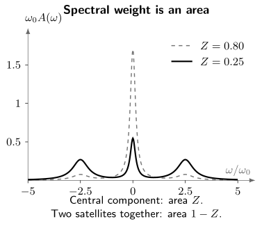
The normalized Lorentzian model in Exercise 4, with $\eta=0.15\omega_0$, $\Gamma=0.45\omega_0$ and satellite centers $\pm2.5\omega_0$. Both spectra have total area one over all frequencies. The central component has area $Z$, not height $Z$; its height also depends on its width. These illustrative curves are not spectra calculated for a specific material.

Optical data provide a complementary partial sum,

$$W(\Omega_c) = \int_0^{\Omega_c} d\omega\, \sigma_1(\omega).$$

The cutoff $\Omega_c$ must be stated. A lost Drude weight may reappear in a mid-infrared feature or in higher interband structure. Matrix elements, multiple orbitals and temperature-dependent lattice effects complicate the comparison. A changing partial integral is not a violation of the full optical sum rule. Broad frequency coverage helps distinguish redistribution from an apparent loss outside the measured window (Basov and collaborators, 2011).

This redistribution distinguishes a correlated evolution from a simple rigid-band picture, but it is not unique to a single microscopic model. Coupling to phonons produces satellites; disorder broadens and localizes; density-wave order reconstructs bands. The strongest diagnosis combines one-particle spectra with charge, spin, optical, and thermodynamic information.

Emergent Degrees of Freedom

An emergent degree of freedom is a variable that efficiently describes the low-energy sector but is not a freely propagating constituent of the microscopic Hamiltonian. Strong correlations often create such variables by freezing some fluctuations and retaining others.

Localized charge can leave spin or orbital moments; a coherent Kondo lattice supports heavy quasiparticles; paired fermions have collective phase fluctuations and Bogoliubov excitations. These are different reductions of the microscopic dynamics. Quantum Spin Liquids and Fractionalization examine more radical possibilities in which excitations belong to distinct deconfined sectors.

Fractionalization is a stronger claim than “the electron is dressed.” An electron-like Landau quasiparticle retains the electron’s conserved quantum-number sector with renormalized overlap. Fractionalized excitations separate those quantum numbers or introduce new topological sectors, and they require evidence for deconfinement rather than a suggestive continuum alone.

Emergence also occurs without exotic fractionalization. Screening converts a bare Coulomb interaction into collective dielectric response. Local moments interact through exchange. A Fermi surface organizes low-temperature thermodynamics even though it is a many-electron object. Anderson’s maxim that “more is different” is useful precisely when it is read as a demand for a correct effective description, not as permission to detach phenomenology from microscopic constraints.

Comparing a model with a material

Several complementary measurements are needed because different mechanisms can produce similar anomalies.

Establish the noninteracting baseline

Determine composition, valence, crystal structure, dimensionality, carrier density, and orbital content. Compare several electronic-structure approximations where possible. State whether the baseline predicts a metal, band insulator, semimetal, or ordered state and which observable it fails to reproduce.

Kohn–Sham eigenvalues are not exact excitation energies, and a failed semilocal functional is not itself proof of Mott physics. Structural errors, magnetic order, spin–orbit coupling, nonlocal exchange, and an incomplete orbital window can change the baseline.

Reconstruct dynamics over a wide window

Photoemission and tunneling constrain occupied or local spectral weight; inverse probes access addition spectra; optical spectroscopy follows current-carrying weight; resonant x-ray and neutron methods probe orbital, charge, and spin sectors. A narrow energy window can mistake a pseudogap, hybridization gap, density-wave gap, or surface feature for a universal correlation gap.

Thermodynamics and response

Specific heat, compressibility, magnetic susceptibility, entropy, charge stiffness, and transport test different parts of the effective theory. Large linear specific heat can indicate a heavy mass, but phonons and nuclear terms must be removed. Bad-metal resistivity can signal loss of coherent transport, but saturation, inhomogeneity, and multiband conduction matter. Linear-in-temperature resistivity is not a standalone definition of strong correlation or “Planckian” dynamics.

Observation	What else can produce it?
Large effective mass	A flat bare band or electron–phonon dressing
Broad or missing spectral peak	Disorder, matrix elements or finite resolution
Insulation at partial band filling	Symmetry breaking, structural change or localization
Mid-infrared optical weight	Interband transitions or polaron absorption
Fluctuating local moments	Dilute impurities or mixed valence
A scattering continuum	Ordinary multiparticle excitations or decay

The material diagnosis should survive tuning. Pressure often increases hopping and bandwidth; doping changes filling and screening; magnetic field changes spin and orbital scales; strain changes geometry and crystal fields. A model becomes more convincing when the same parameters explain several trends without being independently refitted for every observable.

Example: local moments in a two-site singlet

Two sites already illustrate how charge fluctuations and spin dynamics separate. Take two electrons with hopping $t>0$ and repulsion $U\geq0$:

$$H=-t\sum_\sigma(c_{1\sigma}^\dagger c_{2\sigma}+c_{2\sigma}^\dagger c_{1\sigma}) +U\sum_{i=1}^2n_{i\uparrow}n_{i\downarrow}.$$

The singlet ground-state energy is $E_s=(U-\sqrt{U^2+16t^2})/2$ and the triplet energy is zero. The Hubbard dimer derives the exact spectrum. For our purpose, use the Hellmann–Feynman derivative: $\partial_U E_s$ is the total double occupancy, so the occupancy per site is

$$D=\frac12\frac{\partial E_s}{\partial U} =\frac14\left(1-\frac{U}{\sqrt{U^2+16t^2}}\right).$$

At $U=0$, $D=1/4$. At $U=8t$, $D\simeq0.0264$ and $m_{\mathrm{loc}}^2=1-2D\simeq0.947$. The large local fluctuation coexists with a total-spin singlet and $\langle S_i^z\rangle=0$: local moments do not require a nonzero ordered moment.

The singlet–triplet gap, with its large-$U/t$ expansion, is

$$\Delta_{st}=\frac{\sqrt{U^2+16t^2}-U}{2} =\frac{4t^2}{U}+O(t^4/U^3).$$

At $U=8t$, its exact value $0.472t$ is close to the leading exchange estimate $0.500t$. Increasing $U$ suppresses charge fluctuations but also lowers the spin scale. A two-site system does not establish a bulk Mott phase; it isolates the local mechanism before lattice geometry and collective order enter.

Why Strong-Correlation Problems Are Hard

For $N$ spinful orbitals, the full Fock space has dimension

$$\dim\mathcal H = 4^N.$$

The kinetic term is simplest in momentum space, local interactions in real space, and neither basis diagonalizes the full problem. Fermionic signs, frustration, long-range entanglement, low coherence scales, and competing nearly degenerate phases make both analysis and numerics difficult. Real-frequency experiments add an inverse problem because many finite-temperature methods work in imaginary time.

Different methods control different approximations. Exact diagonalization controls a finite cluster; Monte Carlo can control statistical and size errors in favorable sign regimes; tensor networks control entanglement truncation; dynamical mean-field theory treats local temporal fluctuations while approximating spatial correlations. Computational Quantum Matter explains how to choose and compare them. LeBlanc and collaborators (2015) show why independent methods and size extrapolation remain valuable even for the simple square-lattice Hubbard model.

Exercises

1. Double occupancy and local moments

At half filling, evaluate $m_{\mathrm{loc}}^2=\langle n_i\rangle-2D$ for an uncorrelated paramagnet with $D=1/4$ and for an ideal singly occupied limit with $D=0$. Interpret the change.

Solution

At half filling, $\langle n_i\rangle=1$. For independent up and down occupations,

$$m_{\mathrm{loc}}^2 = 1 - 2\left( \frac{1}{4} \right) = \frac{1}{2}.$$

In the singly occupied limit,

$$m_{\mathrm{loc}}^2 = 1.$$

Repulsion suppresses empty–double fluctuations and makes a spinful singly occupied state more probable. This establishes local-moment amplitude, not long-range magnetic order.

2. Residue and width

Suppose near the Fermi level

$$\Sigma^R(\omega) = \Sigma_0 + \left( 1-Z_0^{-1} \right) \hbar\omega - i\gamma,$$

with real $\Sigma_0$, $0<Z_0\le1$, and $\gamma>0$. Find the quasiparticle residue and the renormalized width.

Solution

The derivative of the real self-energy is

$$\frac{\partial \operatorname{Re}\Sigma^R }{ \partial(\hbar\omega) } = 1-Z_0^{-1},$$

so

$$Z = \left[ 1- \left( 1-Z_0^{-1} \right) \right]^{-1} = Z_0.$$

The pole denominator can be multiplied by $Z_0$, showing that the renormalized half-width is

$$\Gamma^\star = Z_0\gamma.$$

A small residue does not automatically make the pole broad. For a low-temperature excitation away from the Fermi surface, compare $\Gamma^\star$ with its excitation energy; near the Fermi surface, temperature and experimental resolution also determine what can be resolved. A finite constant $\gamma$ here describes a local spectral window, not the asymptotic clean Fermi-liquid scattering law.

3. Pressure and a correlation ratio

A one-band fit gives $U=4.0\,\mathrm{eV}$ and $W=2.0\,\mathrm{eV}$ at ambient pressure. Under pressure, assume $U=3.8\,\mathrm{eV}$ and $W=3.0\,\mathrm{eV}$. Compute $U/W$ and explain what can and cannot be concluded.

Solution

The ratios are

$$\left. \frac{U}{W} \right|_{P=0} = 2.0, \qquad \left. \frac{U}{W} \right|_{P} \approx 1.27.$$

Pressure moves this model toward greater itinerancy. The numbers do not by themselves locate a phase boundary. One still needs filling, orbital degeneracy, magnetic and structural order, temperature, longer-range interactions, and the downfolding convention. Spectral, transport, and thermodynamic evolution must test the proposed trend.

4. Conserved spectral weight

Model a momentum-resolved spectrum as

$$A(\omega) ={} ZL_\eta(\omega) + \frac{1-Z}{2} \left[ L_\Gamma(\omega-\Omega) + L_\Gamma(\omega+\Omega) \right],$$

where $L_a(x)=a/[\pi(x^2+a^2)]$ integrates to one. Verify the sum rule and identify the coherent and incoherent weights.

Solution

Integrating term by term gives

$$\int d\omega\,A(\omega) = Z + \frac{1-Z}{2} \left( 1+1 \right) = 1.$$

The central coherent feature carries weight $Z$. The two incoherent satellites together carry $1-Z$. Correlations redistribute weight without violating the single-orbital sum rule. In a real multiorbital experiment, matrix elements and a finite energy window complicate this direct partition.

5. Mott or Slater?

A half-filled material becomes antiferromagnetic and insulating at the same temperature. List measurements that would help distinguish a correlation-driven local-moment insulator from a weak-coupling Slater insulator.

Solution

Useful tests include whether a charge gap or pseudogap persists above the ordering temperature, whether local moments and substantial magnetic entropy exist above it, whether optical weight moves over an interaction-scale window, whether the gap follows the magnetic order parameter, and whether realistic ordered band theory reproduces both charge and spin scales. Pressure or frustration that suppresses order is particularly informative. The two mechanisms can interpolate or coexist, so the goal is a quantitative hierarchy of scales rather than a forced binary label.

References

• P. W. Anderson, “More is different,” Science 177, 393–396 (1972).
• A. Auerbach, Interacting Electrons and Quantum Magnetism, Springer (1994).
• D. N. Basov, R. D. Averitt, D. van der Marel, M. Dressel, and K. Haule, “Electrodynamics of correlated electron materials,” Reviews of Modern Physics 83, 471–541 (2011).
• P. Coleman, Introduction to Many-Body Physics, Cambridge University Press (2015).
• A. Georges, G. Kotliar, W. Krauth, and M. J. Rozenberg, “Dynamical mean-field theory of strongly correlated fermion systems and the limit of infinite dimensions,” Reviews of Modern Physics 68, 13–125 (1996).
• A. Georges, L. de’ Medici, and J. Mravlje, “Strong correlations from Hund’s coupling,” Annual Review of Condensed Matter Physics 4, 137–178 (2013).
• M. Imada, A. Fujimori, and Y. Tokura, “Metal-insulator transitions,” Reviews of Modern Physics 70, 1039–1263 (1998).
• J. P. F. LeBlanc et al., “Solutions of the two-dimensional Hubbard model: Benchmarks and results from a wide range of numerical algorithms,” Physical Review X 5, 041041 (2015).
• M. Troyer and U.-J. Wiese, “Computational complexity and fundamental limitations to fermionic quantum Monte Carlo simulations,” Physical Review Letters 94, 170201 (2005).