Gaussian Channels

A Gaussian channel is a continuous-variable quantum channel that maps Gaussian states to Gaussian states. For bosonic modes, it is the natural channel class for linear optics, attenuation, phase-insensitive amplification, additive Gaussian noise, thermal oscillator damping, and many input–output models before conditioning on non-Gaussian measurement records.

The power of Gaussian channels is that their action on first moments and covariance matrices is finite-dimensional:

$$d \longmapsto Xd+d_0, \qquad V \longmapsto XVX^{\mathsf T}+Y.$$

The real matrices $X,Y$ and displacement $d_0$ specify the channel. They cannot be chosen arbitrarily: complete positivity sets a minimum noise level.

Helpful background. Gaussian States explains first moments and covariance matrices. Erasure and Loss Channels gives the beam-splitter model of attenuation.

Quadratures and vacuum fluctuations

For one mode,

$$q = \frac{a+a^\dagger}{\sqrt2}, \qquad p = \frac{a-a^\dagger}{i\sqrt2}, \qquad [q,p]=i.$$

For $N$ modes, collect quadratures as

$$R = (q_1,p_1,\ldots,q_N,p_N)^{\mathsf T}.$$

The canonical commutation relations are

$$[R_j,R_k] = i\Omega_{jk},$$

with

$$\Omega = \bigoplus_{\ell=1}^N \begin{pmatrix} 0&1\\ -1&0 \end{pmatrix}.$$

The first moments and covariance matrix are

$$d_j=\langle R_j\rangle,$$

and

$$V_{jk} = \frac12 \left\langle \Delta R_j\Delta R_k+\Delta R_k\Delta R_j \right\rangle, \qquad \Delta R_j=R_j-d_j.$$

With this convention, the vacuum covariance of one mode is

$$V_0=\frac12 I_2,$$

and physical covariance matrices satisfy

$$V+\frac{i}{2}\Omega\ge0.$$

All formulas below use this convention. Other communities absorb factors of $2$ or $\hbar$ differently, so covariance noise terms must always be translated with care.

Definition by First and Second Moments

An $N$-mode Gaussian channel acts on first moments and covariance matrices as

$$d' = Xd+d_0,$$

and

$$V' = XVX^{\mathsf T}+Y,$$

where:

• $X$ is a real $2N\times2N$ matrix;
• $d_0$ is a real displacement vector;
• $Y$ is a real symmetric $2N\times2N$ matrix;
• the pair $(X,Y)$ obeys the complete-positivity condition below.

The displacement $d_0$ changes first moments but does not affect noise or complete positivity. The matrix $X$ describes attenuation, amplification, rotations, squeezing, and mode mixing. The matrix $Y$ is the added noise.

For Gaussian inputs, $d$ and $V$ determine the full output state. A precise definition on arbitrary inputs uses $\chi_\rho(k)=\operatorname{Tr}[\rho e^{ik^{\mathsf T}R}]$:

$$\chi_{\Phi(\rho)}(k)=\chi_\rho(X^{\mathsf T}k) \exp\!\left[-\frac12k^{\mathsf T}Yk+ik^{\mathsf T}d_0\right].$$

For non-Gaussian inputs with finite second moments, the moment formulas still hold, but do not determine the full output state. Specifying only the evolution of two moments would not define the channel on arbitrary inputs.

We use equal input and output mode counts below. For $N$ input and $M$ output modes, $X$ is $2M\times2N$, and the positivity condition uses $\Omega_{\mathrm{out}}-X\Omega_{\mathrm{in}}X^{\mathsf T}$.

Complete Positivity

With the convention $V+i\Omega/2\ge0$, the Gaussian map is completely positive if and only if

$$Y+\frac{i}{2} \left( \Omega-X\Omega X^{\mathsf T} \right) \ge0.$$

This condition is the continuous-variable analogue of Choi positivity. It says that the added noise must be large enough to compensate for any change in the commutation-preserving structure caused by $X$.

Important special cases:

• If $X$ is symplectic, so $X\Omega X^{\mathsf T}=\Omega$, the condition reduces to $Y\ge0$.
• A Gaussian unitary has $X$ symplectic and $Y=0$.
• Attenuation and amplification are not arbitrary scalings; quantum mechanics fixes a minimum amount of noise.

For a phase-insensitive one-mode map with $X=\sqrt\tau I_2$, $Y=\nu I_2$, and $\tau\ge0$, the two eigenvalues of this Hermitian matrix are $\nu\pm(1-\tau)/2$. Therefore

$$\nu\ge\frac{|1-\tau|}{2}.$$

Noise is required for both attenuation ($\tau<1$) and amplification ($\tau>1$). At $\tau=1$, additive noise is allowed but not compulsory.

Testing only isolated Gaussian inputs can miss this constraint. For example, the proposed noiseless gain $V\mapsto GV$, $G>1$, preserves their uncertainty condition: $GV+i\Omega/2=(V+i\Omega/2)+(G-1)V\ge0$. Yet it can violate uncertainty when applied to one mode of an entangled pair. The second exercise gives a finite-energy example; no infinitely squeezed reference is needed.

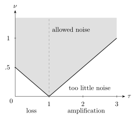
For $X=\sqrt\tau I_2$ and $Y=\nu I_2$, complete positivity permits the shaded region. The boundary $\nu=|1-\tau|/2$ gives vacuum-environment loss and amplification in the convention $V_{\mathrm{vac}}=I_2/2$.

Gaussian Unitary Channels

A Gaussian unitary is generated by a Hamiltonian at most quadratic in the quadratures. It acts as

$$d \longmapsto Sd+d_0, \qquad V \longmapsto SVS^{\mathsf T},$$

where $S$ is symplectic:

$$S\Omega S^{\mathsf T} = \Omega.$$

Examples include:

• phase-space displacements;
• phase rotations of a mode;
• beam splitters;
• single-mode squeezers;
• two-mode squeezers;
• general linear-optical transformations.

These channels are reversible and add no noise. They are the continuous-variable analogue of unitary channels in finite dimensions.

Attenuation and Pure Loss

The one-mode attenuator with transmissivity $\eta$ has

$$0\le\eta\le1, \qquad X=\sqrt{\eta}\,I_2.$$

For an independent, centered Gaussian environment of covariance $V_E$, the beam-splitter dilation gives

$$d \longmapsto \sqrt{\eta}\,d, \qquad V \longmapsto \eta V+(1-\eta)V_E.$$

For a vacuum environment,

$$V_E=\frac12 I_2,$$

so

$$V' = \eta V+\frac{1-\eta}{2}I_2.$$

This is the quantum-limited pure-loss channel. It is the covariance-matrix form of the beam-splitter loss model discussed in Erasure and Loss Channels.

The added vacuum term is not optional. If one tried to map $V\mapsto\eta V$ with no environmental contribution, the vacuum would be sent to $\eta I_2/2$, violating the uncertainty principle for $\eta\lt1$.

Serial pure-loss channels multiply transmissivities; the discrete-time composition viewpoint is collected in Channel Composition and Fixed Points.

Thermal-Loss Channel

For a thermal environment with mean occupation $\bar n_E$,

$$V_E = \left( \bar n_E+\frac12 \right)I_2.$$

The thermal-loss channel is therefore

$$V' = \eta V + (1-\eta) \left( \bar n_E+\frac12 \right)I_2.$$

Quantum Illumination uses noisy attenuation to compare target-presence and target-absence hypotheses.

It has the thermal covariance as a fixed point:

$$V=V_E \quad\Longrightarrow\quad V'=V_E.$$

For a constant-rate oscillator damping model in the rotating frame,

$$\eta(t)=e^{-\kappa t}.$$

The bath occupation $\bar n_E$ is set by the environment temperature and oscillator frequency. At optical frequencies, vacuum loss is often a good approximation; at microwave frequencies, thermal occupation can be important.

Phase-Insensitive Amplification

A phase-insensitive amplifier with gain $G\ge1$ has

$$X=\sqrt G\,I_2.$$

A two-mode squeezing dilation has

$$a_{\mathrm{out}}=\sqrt G\,a_{\mathrm{in}}+\sqrt{G-1}\,e_{\mathrm{in}}^\dagger.$$

The creation operator is essential: $[a_{\mathrm{out}},a_{\mathrm{out}}^\dagger]=G-(G-1)=1$. For an independent centered environment of covariance $V_E$,

$$d'=\sqrt G\,d,\qquad V'=GV+(G-1)ZV_EZ,\qquad Z=\operatorname{diag}(1,-1).$$

The $Z$ matrices reflect the sign reversal of the environment momentum in $e^\dagger$. For a thermal environment $ZV_EZ=V_E$, and the added noise is isotropic. A squeezed environment need not give phase-insensitive noise. For a quantum-limited amplifier,

$$V_E=\frac12I_2,$$

and therefore

$$V' = GV+\frac{G-1}{2}I_2.$$

The added-noise term is required by complete positivity. Without it, the map would scale both quadratures by $\sqrt G$ while also amplifying commutators incorrectly. Physically, a phase-insensitive amplifier must add at least vacuum noise.

Phase-sensitive amplification is different: squeezing can amplify one quadrature while deamplifying the conjugate quadrature through a Gaussian unitary. The noise bound above concerns deterministic phase-insensitive gain.

Additive Gaussian Noise

An additive Gaussian-noise channel leaves the first moments unchanged and adds classical displacement noise:

$$d \longmapsto d, \qquad V \longmapsto V+N,$$

with

$$N=N^{\mathsf T}\ge0.$$

This is the Gaussian channel with $X=I$ and $Y=N$. The complete-positivity condition reduces to $N\ge0$.

A physical picture is random displacement:

$$\rho \longmapsto \int d^{2N}\xi\, P(\xi) D(\xi)\rho D(\xi)^\dagger,$$

Here $P(\xi)$ is a centered classical Gaussian distribution, and $D(\xi)^\dagger R D(\xi)=R+\xi$. If $P$ has covariance $N$, the covariance matrix gains $N$ in the same convention.

Additive noise models technical displacement noise, classical Gaussian backgrounds, and some effective limits of thermal or electronic noise. It is not the same as photon loss: loss attenuates first moments, while additive noise does not.

Multimode Form

For several modes, the same formula

$$V' = XVX^{\mathsf T}+Y$$

allows mode mixing, correlated noise, and loss to several environments. A passive linear-optical network retaining all its modes is symplectic and orthogonal, so it has $Y=0$. Discarding output modes instead gives a noisy reduced channel. Independent loss on each mode has

$$X = \bigoplus_{j=1}^N \sqrt{\eta_j}\,I_2,$$

and

$$Y = \bigoplus_{j=1}^N (1-\eta_j) \left( \bar n_j+\frac12 \right)I_2.$$

Correlated Gaussian noise has off-diagonal blocks in $Y$. Such correlations matter in multimode sensing, communication, and oscillator networks.

A squeezed input through loss

Take a centered squeezed vacuum with $V=\operatorname{diag}(1/8,2)$. Its determinant is $1/4$, saturating the uncertainty relation. Pure loss with $\eta=1/2$ gives

$$V'=\frac12V+\frac14 I_2 =\operatorname{diag}(5/16,5/4).$$

The initially squeezed variance rises toward $1/2$, while the initially large variance falls toward $1/2$. Thus attenuation need not increase every variance. The determinant becomes $25/64$, so the state becomes mixed: the one-mode Gaussian purity is $1/(2\sqrt{\det V'})=4/5$.

For vacuum input, pure loss leaves $V=I_2/2$ unchanged. A quantum-limited amplifier with $G=2$ instead sends that vacuum to $V'=3I_2/2$, a thermal state with mean photon number one. These checks distinguish attenuation from amplification even when both scale a signal.

Gaussian channels arise by coupling initially independent system and Gaussian environment modes through a Gaussian unitary, then tracing out the environment. The environmental noise is part of the physical operation, even when the first-moment equation contains only a simple scaling.

What Gaussian Channels Do Not Cover

Gaussian channels do not include every important continuous-variable process. Non-Gaussian processes include:

• photon counting with conditioning;
• photon subtraction or addition;
• Kerr nonlinearities;
• threshold detectors as state-update maps;
• finite-dimensional truncation artifacts;
• loss conditioned on a number-resolved environment record;
• non-Gaussian noise distributions;
• general random phase rotations, even if the random phase has a Gaussian distribution.

Random phase rotation is not additive displacement noise. Uniformly randomizing the phase of a nonzero coherent state produces a Poisson-distributed number-diagonal state, not a thermal Gaussian state. A small phase fluctuation around a large coherent amplitude can sometimes be approximated by displacement noise, but that requires linearization.

Also, a Gaussian channel acting on a non-Gaussian input generally produces an output whose full state is not determined by $d$ and $V$ alone. Moment formulas remain useful, but they do not replace the density operator.

Continuous-Variable Quantum Computation explains the use and limits of Gaussian operations in computation.

Exercises

1. Pure-loss vacuum check. Show that the pure-loss channel maps the vacuum covariance $I_2/2$ to itself.

Solution

For pure loss,

$$V' = \eta V+\frac{1-\eta}{2}I_2.$$

Set $V=I_2/2$:

$$V' = \eta\frac{I_2}{2} + \frac{1-\eta}{2}I_2 = \frac12I_2.$$

Thus vacuum is a fixed point of quantum-limited attenuation.

2. An entangled input detects missing amplifier noise. In the order $(q_A,p_A,q_B,p_B)$, take the centered two-mode Gaussian input

$$V_{AB}=\begin{pmatrix}I_2&\frac{\sqrt3}{2}Z\\\frac{\sqrt3}{2}Z&I_2\end{pmatrix}, \qquad Z=\operatorname{diag}(1,-1).$$

Identify it as a physical two-mode squeezed state. Apply the proposed gain $X_A=\sqrt2 I_2$, $Y_A=0$ to $A$, leaving $B$ untouched. Show that the joint output fails $V'_{AB}+i(\Omega\oplus\Omega)/2\ge0$, although both one-mode outputs satisfy uncertainty. What noise restores a physical amplifier?

Solution

This is the two-mode squeezed covariance with $\cosh2r=2$ and $\sinh2r=\sqrt3$. It is pure, normalizable, and has mean occupation $1/2$ per mode. Applying $X_A\oplus I_2$ gives

$$V'_{AB}=\begin{pmatrix}2I_2&\frac{\sqrt6}{2}Z\\\frac{\sqrt6}{2}Z&I_2\end{pmatrix}.$$

The marginals $2I_2$ and $I_2$ separately satisfy uncertainty. For the joint test, put $e_\pm=(1,\pm i)^{\mathsf T}/\sqrt2$. In the orthonormal subspace spanned by $(e_-,0)$ and $(0,e_+)$, the Hermitian uncertainty matrix restricts to

$$\begin{pmatrix}5/2&\sqrt6/2\\\sqrt6/2&1/2\end{pmatrix}.$$

Its determinant is $-1/4$, so it has a negative eigenvalue. The proposed joint output is not a quantum state; this is failure of positivity, not merely a change in entanglement.

The quantum-limited gain-$2$ amplifier adds $Y_A=I_2/2$ on $A$. Then the displayed restriction becomes $\begin{pmatrix}3&\sqrt6/2\\\sqrt6/2&1/2\end{pmatrix}$, which is positive with determinant zero; the complementary orthogonal subspace is positive too. More generally, $Y_A=(G-1)I_2/2$ satisfies the complete-positivity inequality and works for every joint input. These are precisely the vacuum fluctuations supplied by the amplifier’s environment.

3. Thermal fixed point. Show that the thermal-loss map has $V_E=(\bar n_E+1/2)I_2$ as a fixed covariance matrix.

Solution

The thermal-loss covariance map is

$$V' = \eta V+(1-\eta)V_E.$$

Set $V=V_E$:

$$V' = \eta V_E+(1-\eta)V_E = V_E.$$

Thus $V_E$ is fixed. For repeated applications with $0\le\eta<1$, $V_n-V_E=\eta^n(V_0-V_E)$ tends to zero; $\eta=1$ instead gives the identity channel.

4. Additive noise is not loss. Compare the transformations of first moments under pure loss and additive Gaussian noise.

Solution

Pure loss gives

$$d\mapsto\sqrt{\eta}\,d,$$

so displacements are attenuated. Additive Gaussian noise gives

$$d\mapsto d,$$

so the mean displacement is unchanged. Both can increase uncertainty, but only attenuation reduces the signal amplitude.

References

• A. S. Holevo and R. F. Werner, “Evaluating capacities of bosonic Gaussian channels,” Physical Review A 63, 032312 (2001). DOI; author manuscript.
• C. Weedbrook, S. Pirandola, R. García-Patrón, N. J. Cerf, T. C. Ralph, J. H. Shapiro, and S. Lloyd, “Gaussian quantum information,” Reviews of Modern Physics 84, 621–669 (2012). DOI; author manuscript. The review uses vacuum covariance $I$; divide its covariances and added-noise matrices by two to obtain the convention here.