Pauli Channels

A Pauli channel is a stochastic mixture of conjugations by Pauli operators. For one qubit,

$$\Phi(\rho) = p_0\rho + p_1X\rho X + p_2Y\rho Y + p_3Z\rho Z, \qquad p_\mu\ge0, \quad \sum_{\mu=0}^3p_\mu=1.$$

Equivalently,

$$\Phi(\rho) = \sum_{\mu=0}^3 p_\mu\sigma_\mu\rho\sigma_\mu, \qquad \sigma_0=I,\quad \sigma_1=X,\quad \sigma_2=Y,\quad \sigma_3=Z.$$

Pauli channels are useful because they are completely positive, trace preserving, unital, diagonal in the Pauli operator basis, and compatible with stabilizer and error-correction calculations. They cannot describe nonunital relaxation, leakage from the modeled space, or a general coherent overrotation. Correlated errors, however, can be Pauli errors: the Pauli labels on different qubits need not be independent.

Helpful background. Pauli Matrices supplies the conjugation identities used below; the Bloch sphere turns these matrix operations into changes of three real coordinates.

Channel and Kraus Form

The Kraus operators may be chosen as

$$K_\mu = \sqrt{p_\mu}\,\sigma_\mu, \qquad \mu=0,1,2,3.$$

The trace-preserving condition is immediate:

$$\sum_{\mu=0}^3 K_\mu^\dagger K_\mu = \sum_{\mu=0}^3 p_\mu I = I.$$

The channel is also unital:

$$\Phi(I) = \sum_{\mu=0}^3 p_\mu\sigma_\mu I\sigma_\mu = I.$$

Thus a Pauli channel is a random unitary channel. One pure-environment representation is:

$$V\lvert\psi\rangle = \sum_{\mu=0}^3 \sqrt{p_\mu}\, \sigma_\mu\lvert\psi\rangle \otimes \lvert\mu\rangle_E.$$

This isometry can entangle the system and environment; it is not itself a classical mixture. Measuring the environment in the $|\mu\rangle_E$ basis produces a classical record. If that record is available, the receiver can apply $\sigma_\mu$ again to undo the error. If the record is ignored, the reduced system state undergoes the Pauli channel. This is a simple example of a Stinespring representation.

Bloch-Vector Action

Write a qubit density operator as

$$\rho = \frac12 \left( I+r_xX+r_yY+r_zZ \right).$$

Conjugation by $X$ preserves the $X$ component and flips the $Y$ and $Z$ components:

$$X\rho X = \frac12 \left( I+r_xX-r_yY-r_zZ \right).$$

Similarly, $Y$ preserves $r_y$ and flips $r_x,r_z$, while $Z$ preserves $r_z$ and flips $r_x,r_y$. Therefore a Pauli channel acts diagonally on the Bloch vector:

$$(r_x,r_y,r_z) \longmapsto (\lambda_xr_x,\lambda_yr_y,\lambda_zr_z),$$

where

$$\begin{aligned} \lambda_x&=p_0+p_1-p_2-p_3,\\ \lambda_y&=p_0-p_1+p_2-p_3,\\ \lambda_z&=p_0-p_1-p_2+p_3. \end{aligned}$$

The origin of the Bloch ball is fixed because the channel is unital. The three axes may contract by different factors and may also acquire sign flips when an eigenvalue is negative.

This diagonal form is one reason Pauli channels are analytically convenient: they turn many channel calculations into three scalar eigenvalue calculations.

Complete-Positivity Tetrahedron

Conversely, a trace-preserving unital qubit map that is diagonal in the Pauli basis has the form

$$(r_x,r_y,r_z) \mapsto (\lambda_xr_x,\lambda_yr_y,\lambda_zr_z).$$

It is a Pauli channel exactly when the probabilities obtained by inversion are nonnegative:

$$\begin{aligned} p_0&=\frac{1+\lambda_x+\lambda_y+\lambda_z}{4},\\ p_1&=\frac{1+\lambda_x-\lambda_y-\lambda_z}{4},\\ p_2&=\frac{1-\lambda_x+\lambda_y-\lambda_z}{4},\\ p_3&=\frac{1-\lambda_x-\lambda_y+\lambda_z}{4}. \end{aligned}$$

Complete positivity is therefore equivalent to the four inequalities

$$\begin{array}{rcl} 1+\lambda_x+\lambda_y+\lambda_z&\ge&0,\\ 1+\lambda_x-\lambda_y-\lambda_z&\ge&0,\\ 1-\lambda_x+\lambda_y-\lambda_z&\ge&0,\\ 1-\lambda_x-\lambda_y+\lambda_z&\ge&0. \end{array}$$

These inequalities form a tetrahedron inside the cube $[-1,1]^3$. Positivity of the map on isolated qubit states only gives the cube; complete positivity gives the smaller tetrahedron. This is a useful concrete example of the distinction explained in Completely Positive Maps.

For example, $(\lambda_x,\lambda_y,\lambda_z)=(0.5,0.3,0.4)$ gives probabilities $(0.55,0.20,0.10,0.15)$. All four are nonnegative. In contrast, $(1,1,0.4)$ still maps the isolated Bloch ball into itself, but gives $p_3=-0.15$: applying this map to half of a Bell pair would give a negative eigenvalue.

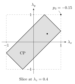
At fixed $\lambda_z=0.4$, positivity permits the dashed square. Complete positivity permits only the shaded diamond, where all four $p_\mu$ are nonnegative. The point $(1,1)$ fails the Bell-pair test. This is a slice of the three-dimensional tetrahedron, not the full set.

Choi Matrix

Using the output-input convention of Choi Matrix, a Pauli channel has

$$J_\Phi = \sum_{\mu=0}^3 p_\mu \lvert\sigma_\mu\rangle\rangle \langle\langle\sigma_\mu\rvert,$$

where $\lvert A\rangle\rangle$ is the vectorized operator in the chosen input basis.

For one qubit, the four normalized vectors

$$\frac{1}{\sqrt2} \lvert\sigma_\mu\rangle\rangle$$

are Bell states up to phases. Thus the normalized Choi state is Bell diagonal, with eigenvalues $p_\mu$:

$$\tau_\Phi = \frac12J_\Phi, \qquad \operatorname{spec}(\tau_\Phi) = \{p_0,p_1,p_2,p_3\}.$$

The Choi matrix makes complete positivity transparent: these eigenvalues must be nonnegative. The number of nonzero $p_\mu$ is the Choi rank and hence the minimum number of Kraus operators.

Special Cases

Phase-flip and dephasing channel

The $Z$ phase-flip channel is

$$\Phi_p(\rho) = (1-p)\rho+pZ\rho Z.$$

It is a Pauli channel with

$$p_0=1-p,\qquad p_3=p,\qquad p_1=p_2=0.$$

Its Bloch eigenvalues are

$$\lambda_x=\lambda_y=1-2p, \qquad \lambda_z=1.$$

It preserves populations in the $Z$ basis and multiplies transverse coherences by $1-2p$. Their magnitude vanishes at $p=1/2$ and returns to its original value at the unitary endpoint $p=1$. This is the Pauli-channel form of Dephasing Channel.

Bit-flip and bit-phase-flip channels

The $X$ bit-flip channel

$$\Phi_p(\rho) = (1-p)\rho+pX\rho X$$

has

$$\lambda_x=1, \qquad \lambda_y=\lambda_z=1-2p.$$

The $Y$ bit-phase-flip channel is analogous, preserving the $Y$ component and damping the $X$ and $Z$ components.

These names are basis dependent. They are useful in qubit error models, but they should not be mistaken for basis-independent physical mechanisms.

Depolarizing channel

The qubit Pauli-error convention for depolarizing noise is

$$\mathcal P_p(\rho) = (1-p)\rho + \frac{p}{3} \left( X\rho X+Y\rho Y+Z\rho Z \right).$$

Thus

$$p_0=1-p, \qquad p_1=p_2=p_3=\frac{p}{3}.$$

All Bloch eigenvalues are equal:

$$\lambda_x=\lambda_y=\lambda_z = 1-\frac{4p}{3}.$$

The replacement-probability convention instead writes

$$\mathcal D_q(\rho) = (1-q)\rho+q\frac{I}{2}.$$

The conversion is

$$q=\frac{4p}{3}.$$

For $q>1$, the map can still be completely positive, but $q$ is no longer a replacement probability. In particular, in the Pauli-error convention, $p=3/4$ gives the completely mixed output, while $p=1$ gives the valid but negative-shrink channel with $\lambda=-1/3$. See Depolarizing Channel for the full parameter map.

Multiqubit Pauli Channels

For $n$ qubits, use Pauli strings

$$P_{\mathbf a} = P_{a_1}\otimes\cdots\otimes P_{a_n}, \qquad P_{a_j}\in\{I,X,Y,Z\},$$

ignoring overall phases. A multiqubit Pauli channel is

$$\Phi(\rho) = \sum_{\mathbf a} p_{\mathbf a} P_{\mathbf a}\rho P_{\mathbf a}, \qquad p_{\mathbf a}\ge0, \quad \sum_{\mathbf a}p_{\mathbf a}=1.$$

An independent one-qubit Pauli noise model is the special case where the distribution factors:

$$p_{\mathbf a} = \prod_{j=1}^n p_{a_j}^{(j)}.$$

Correlated Pauli noise allows arbitrary probabilities $p_{\mathbf a}$. For example, the event $Z_1Z_2$ can occur with a probability not determined by the marginal $Z_1$ and $Z_2$ rates.

This distinction matters for error correction. A code that corrects independent single-qubit errors can behave very differently under spatially correlated Pauli strings. Thus “Pauli channel” does not automatically mean “independent errors.” For the algebraic stabilizer background, see Stabilizer States Preview and Stabilizer Identities.

Pauli Noise and Depolarizing Channels develops propagation through Clifford gates and the resulting syndrome probabilities.

Pauli twirling and repeated coherent errors

Pauli twirling averages a CPTP map over Pauli conjugations. For $n$ qubits,

$$\mathcal T(\Phi)(\rho) =\frac{1}{4^n}\sum_Q Q^\dagger\Phi(Q\rho Q^\dagger)Q,$$

where the sum contains all phase-free $n$-qubit Pauli strings. The resulting channel is diagonal in the Pauli basis: averaging cancels off-diagonal transfer coefficients and any nonunital translation. This is an exact transformation of the specified channel. Replacing an experimental channel by its twirl is justified only when such averaging is performed or when the approximation preserves the quantity of interest.

A worked comparison. A coherent rotation $U=e^{-i\epsilon Z/2}$ has the Pauli twirl

$$\mathcal T(\mathcal U)(\rho) =\cos^2(\epsilon/2)\rho+\sin^2(\epsilon/2)Z\rho Z.$$

For input $|+\rangle$, both maps give $\langle X\rangle=\cos\epsilon$ after one use. After $N$ identical rotations, however,

$$\langle X\rangle_{\mathrm{coherent}}=\cos(N\epsilon), \qquad \langle X\rangle_{\mathrm{independent\ twirls}}=(\cos\epsilon)^N.$$

With $\epsilon=0.1$ radians and $N=10$, these are approximately $0.5403$ and $0.9511$. Agreement for one application does not imply agreement after repeated use. The two infidelities with the initial $|+\rangle$ scale as $N^2\epsilon^2/4$ and $N\epsilon^2/4$, respectively, when $N|\epsilon|\ll1$.

Twirling does not force multiqubit Pauli probabilities to factor: it retains spatially correlated Pauli strings. Modeling them as independent requires another approximation. A one-time twirl also does not specify temporal memory, and twirling within a qubit space cannot repair a model that omits leakage levels.

What Pauli Channels Cannot Model

Pauli channels are unital:

$$\Phi(I)=I.$$

Therefore they cannot model relaxation toward a pure ground state. The Amplitude-Damping Channel is the standard counterexample: it is trace preserving and completely positive, but for $\gamma>0$ it sends $I/2$ toward $\lvert0\rangle\langle0\rvert$.

Pauli channels also preserve the system Hilbert space. They do not describe flagged erasure unless the output space includes a loss flag, and they do not describe leakage unless the Hilbert space is enlarged.

Finally, a coherent unitary error such as

$$\rho \mapsto e^{-i\epsilon Z/2} \rho e^{i\epsilon Z/2}$$

is not generally the same as stochastic $Z$ flips. Coherent errors can accumulate systematically, while stochastic Pauli errors compose probabilistically.

Exercises

1. Bloch eigenvalues. Derive the formulas for $\lambda_x,\lambda_y,\lambda_z$ in terms of $p_0,p_1,p_2,p_3$.

Solution

Use

$$X X X=X,\qquad X Y X=-Y,\qquad X Z X=-Z,$$

and the analogous cyclic identities. The $X$ component of the output receives sign $+1$ from the $I$ and $X$ branches and sign $-1$ from the $Y$ and $Z$ branches:

$$\lambda_x=p_0+p_1-p_2-p_3.$$

Similarly,

$$\lambda_y=p_0-p_1+p_2-p_3, \qquad \lambda_z=p_0-p_1-p_2+p_3.$$

2. Invert the probabilities. Starting from the three $\lambda_i$ equations and $\sum_\mu p_\mu=1$, derive the inverse formulas for $p_\mu$.

Solution

Add the normalization equation to all three eigenvalue equations:

$$1+\lambda_x+\lambda_y+\lambda_z = 4p_0.$$

Changing signs selects the other probabilities:

$$\begin{aligned} 1+\lambda_x-\lambda_y-\lambda_z&=4p_1,\\ 1-\lambda_x+\lambda_y-\lambda_z&=4p_2,\\ 1-\lambda_x-\lambda_y+\lambda_z&=4p_3. \end{aligned}$$

Dividing by $4$ gives the stated inverse formulas. Complete positivity is then $p_\mu\ge0$ for all $\mu$.

3. Dephasing as a Pauli channel. Show that the phase-flip channel $(1-p)\rho+pZ\rho Z$ maps $\rho_{01}$ to $(1-2p)\rho_{01}$.

Solution

For

$$\rho= \begin{pmatrix} \rho_{00}&\rho_{01}\\ \rho_{10}&\rho_{11} \end{pmatrix},$$

one has

$$Z\rho Z = \begin{pmatrix} \rho_{00}&-\rho_{01}\\ -\rho_{10}&\rho_{11} \end{pmatrix}.$$

Therefore

$$\rho_{01}' = (1-p)\rho_{01} -p\rho_{01} = (1-2p)\rho_{01}.$$

4. Why amplitude damping is not Pauli. Use unitality to show that the amplitude-damping channel with $\gamma>0$ cannot be a Pauli channel.

Solution

Every Pauli channel is unital:

$$\Phi(I)=I.$$

For amplitude damping with Kraus operators

$$K_0= \begin{pmatrix} 1&0\\ 0&\sqrt{1-\gamma} \end{pmatrix}, \qquad K_1= \begin{pmatrix} 0&\sqrt{\gamma}\\ 0&0 \end{pmatrix},$$

one finds

$$K_0K_0^\dagger+K_1K_1^\dagger = \begin{pmatrix} 1+\gamma&0\\ 0&1-\gamma \end{pmatrix}.$$

This equals $I$ only when $\gamma=0$. Hence nontrivial amplitude damping is not a Pauli channel.

References

• M. A. Nielsen and I. L. Chuang, Quantum Computation and Quantum Information, 10th anniversary edition, Cambridge University Press (2010).
• M. B. Ruskai, S. Szarek, and E. Werner, “An analysis of completely-positive trace-preserving maps on $M_2$,” Linear Algebra and its Applications 347, 159–187 (2002). DOI; author manuscript.
• J. Watrous, The Theory of Quantum Information, Cambridge University Press (2018). Author’s text.