Unravelings

An unraveling is a representation of an unconditional open-system evolution as an ensemble of conditioned trajectories. The same density matrix $\rho(t)$ can be written as an average over many possible records:

$$\rho(t) = \mathbb E_{\mathcal U} \!\left[ \rho_c^{(\mathcal U)}(t) \right],$$

where $\mathcal U$ labels the monitoring scheme or stochastic representation. Photon counting, homodyne detection, heterodyne detection, and other trajectory constructions can all unravel the same Lindblad master equation.

The main lesson is:

$$\text{the unconditional master equation does not determine a unique record.}$$

To assign operational meaning to a trajectory, specify how the environment or output channel is monitored.

A Fixed Lindblad Generator

Consider a Markovian master equation

$$\frac{d\rho}{dt} = \mathcal L\rho = - \frac{i}{\hbar}[H,\rho] + \sum_k\mathcal D[L_k]\rho,$$

with

$$\mathcal D[L]\rho = L\rho L^\dagger - \frac12\{L^\dagger L,\rho\}.$$

This equation describes the ensemble state when output records are ignored. An unraveling adds a record model and a conditioned update rule such that averaging over records returns the same $\mathcal L$.

The conditional states may be pure or mixed, jump-like or diffusive, smooth between events or noisy at every instant. Those differences are not visible in $\rho(t)$ alone.

Photon-Counting Unraveling

If a channel $L$ is monitored by direct detection, the record is a counting process. The conditional intensity is

$$\mathbb E[dN_t|\rho_c(t)] = \operatorname{Tr}(L^\dagger L\rho_c(t))\,dt$$

for unit efficiency. A click updates the state through the jump operation

$$\rho_c \longmapsto \frac{L\rho_cL^\dagger} {\operatorname{Tr}(L^\dagger L\rho_c)}.$$

No-click intervals are also conditioned evolution. The ensemble of all click and no-click histories recovers the dissipator $\mathcal D[L]\rho$.

The detection model is Photon Counting; the conditioned dynamics is Quantum Jump Trajectories.

Homodyne Unraveling

The same output channel can be mixed with a strong local oscillator and measured as a quadrature. A homodyne record has the schematic form

$$dY_t = \sqrt{\eta}\, \langle e^{-i\phi}L+e^{i\phi}L^\dagger\rangle_c\,dt + dW_t.$$

Changing the local-oscillator phase $\phi$ changes the measured quadrature and therefore changes the individual conditioned trajectories. The unconditional master equation is unchanged after averaging.

Thus the same dissipator $\mathcal D[L]\rho$ can be represented by photon-counting jumps or by homodyne diffusion. Neither trajectory picture is the unique hidden story behind the master equation. Each is tied to a different record.

For the detector model, see Homodyne Detection. For the stochastic equation, see Diffusive Trajectories.

Heterodyne and Other Diffusive Unravelings

Heterodyne detection records two quadratures, often written as a complex record

$$dZ_t = \sqrt{\eta}\,\langle L\rangle_c\,dt + d\zeta_t.$$

It gives a different conditioned ensemble from a fixed-phase homodyne measurement. More generally, diffusive unravelings can involve different quadrature phases, channel mixing, adaptive phases, or inefficient detection. The ensemble average is constrained by the same master equation, but the records and conditioned states differ.

This freedom is useful experimentally and computationally. It is also a warning: a plotted trajectory is not an invariant property of the open system. It is a property of the system plus monitoring scheme.

The Same Dephasing Seen Two Ways

Let $H=0$, $L=\sqrt\gamma\,\sigma_z$, and initially $\rho=\lvert+x\rangle\langle+x\rvert$. The ensemble Bloch coordinate is $x(t)=e^{-2\gamma t}$.

• Count the output. The rate is $\langle L^\dagger L\rangle=\gamma$, independent of the qubit state. Each detected event applies $\sigma_z$, so $x_c(t)=(-1)^{N_t}$. The count reveals which phase flips occurred, but gives no information about $\sigma_z$.
• Measure the informative quadrature. Homodyne detection at phase zero produces $dY=2\sqrt\gamma z_cdt+dW$. The state gradually resolves a $\sigma_z$ eigenstate. For ideal efficiency, $z_c=\tanh(2\sqrt\gamma Y_t)$ and $x_c=\operatorname{sech}(2\sqrt\gamma Y_t)$, as derived in Bayesian Quantum Measurement.

The conditioned states look very different, yet both averages give the same exponential coherence decay. The detector decides what information about the output becomes available.

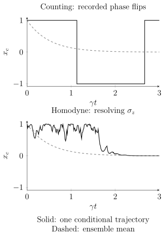
Two illustrative ideal records for $L=\sqrt\gamma\sigma_z$, initially $\lvert+x\rangle$. Solid curves show one conditional $x_c$ in each scheme; dashed curves show the common ensemble mean $e^{-2\gamma t}$. The sample curves are not expected to follow their mean. Both detection schemes retain pure states, with different conditional Bloch vectors.

Channel Mixing

If several Lindblad channels are present, measuring different linear combinations of the output fields can produce different records while leaving the unconditional generator unchanged. For two channels, a unitary mixing

$$M_\alpha = \sum_k u_{\alpha k}L_k, \qquad u^\dagger u=I,$$

satisfies

$$\sum_\alpha \mathcal D[M_\alpha]\rho = \sum_k \mathcal D[L_k]\rho.$$

The master equation does not know which output basis a detector uses. A detector that resolves channels $L_1,L_2$ conditions the state differently from a detector that resolves $M_1,M_2$, even though the unread state can obey the same equation.

This should be distinguished from a mere change of notation. Physical meaning comes from the ports, beam splitters, local oscillators, detector modes, and records.

Simulation Versus Measurement

Unravelings are often used as Monte Carlo simulation tools. One can simulate many pure-state trajectories and average them to approximate a density-matrix master equation. This can be numerically efficient, especially in large Hilbert spaces.

But a simulation trajectory is not automatically an experimental record. It becomes operationally meaningful only if the stochastic process corresponds to a possible monitoring scheme. Without such a scheme, the trajectory is a computational representation of the density matrix, not a directly observed path.

This distinction is especially important in foundations discussions. Quantum trajectories do not add detector-independent hidden paths to the theory. They are conditioned state assignments or stochastic decompositions tied to records.

Efficiency and Unmonitored Channels

An ideal pure-state unraveling usually assumes that every relevant environmental channel is monitored with unit efficiency. If some information is lost, the conditional state generally becomes mixed. A common model splits a channel into monitored and unmonitored parts:

$$L_{\mathrm{mon}} = \sqrt{\eta}\,L, \qquad L_{\mathrm{loss}} = \sqrt{1-\eta}\,L.$$

The two dissipators add to the same total:

$$\mathcal D[L_{\mathrm{mon}}]\rho + \mathcal D[L_{\mathrm{loss}}]\rho = \mathcal D[L]\rho.$$

Only the monitored part appears in the observer’s record. The unmonitored part still causes decoherence or dissipation, so the conditional state contains less information than an ideal trajectory would.

Exercises

1. For one collapse operator $L$, explain why photon counting and homodyne detection can average to the same dissipator while producing different individual trajectories.

Solution

The dissipator $\mathcal D[L]\rho$ describes the unread effect of coupling to the output channel. Photon counting retains event information from that output, while homodyne detection retains quadrature information obtained by interfering the output with a local oscillator. The records are different, so the conditional updates are different. After averaging over all possible records with their correct probabilities, both descriptions erase the record information and recover the same unconditional channel.

2. Let

$$M_1 = \frac{L_1+L_2}{\sqrt2}, \qquad M_2 = \frac{L_1-L_2}{\sqrt2}.$$

Show that $\sum_\alpha M_\alpha\rho M_\alpha^\dagger=\sum_k L_k\rho L_k^\dagger$.

Solution

Compute the two terms:

$$\begin{aligned} M_1\rho M_1^\dagger &= \frac12 (L_1+L_2)\rho(L_1^\dagger+L_2^\dagger), \\ M_2\rho M_2^\dagger &= \frac12 (L_1-L_2)\rho(L_1^\dagger-L_2^\dagger). \end{aligned}$$

Adding them cancels the cross terms and leaves

$$M_1\rho M_1^\dagger + M_2\rho M_2^\dagger = L_1\rho L_1^\dagger + L_2\rho L_2^\dagger.$$

The same cancellation also preserves the anticommutator part because $\sum_\alpha M_\alpha^\dagger M_\alpha=\sum_kL_k^\dagger L_k$.

3. Why does finite efficiency generally make the conditioned state more mixed?

Solution

Finite efficiency means that some information carried away by the environment is not included in the observer’s record. The unobserved part still affects the system through the unconditional dissipator, but the observer cannot condition on its detailed outcome. The conditional state must therefore average over those lost alternatives, which generally produces mixing.

4. A simulation uses quantum jumps to solve a master equation, but the experiment actually measures a homodyne current. Which trajectory picture should be used to interpret a single experimental record?

Solution

The homodyne trajectory picture should be used for the single experimental record, because the actual retained data are a homodyne current. A jump simulation may still be a valid numerical method for the same unconditional master equation, but its individual jumps do not correspond to the observed record unless the environment is actually monitored by photon counting.

References

• H. J. Carmichael, An Open Systems Approach to Quantum Optics, Springer, 1993.
• J. Dalibard, Y. Castin, and K. Mølmer, “Wave-function approach to dissipative processes in quantum optics,” Physical Review Letters 68, 580–583, 1992.
• N. Gisin and I. C. Percival, “The quantum-state diffusion model applied to open systems,” Journal of Physics A 25, 5677–5691, 1992.
• K. Jacobs, Quantum Measurement Theory and its Applications, Cambridge University Press, 2014.
• M. B. Plenio and P. L. Knight, “The quantum-jump approach to dissipative dynamics in quantum optics,” Reviews of Modern Physics 70, 101–144, 1998.
• H. M. Wiseman and G. J. Milburn, Quantum Measurement and Control, Cambridge University Press, 2010.