Subsystem Codes

A subsystem code stores information in one factor of an encoded Hilbert space while allowing another factor, called the gauge subsystem, to change. Gauge measurements can therefore simplify error correction without preserving every encoded degree of freedom. The distinction is physical: changing a gauge qubit is harmless to the protected information; changing a logical qubit is not.

We first make that distinction explicit in four qubits, then develop the Bacon–Shor family and its decoding limits. Low-weight gauge measurements are useful, but neither their weight nor the static code distance determines the reliability of a complete recovery circuit.

Required background. Why Quantum Error Correction Is Possible explains error spans and exact correctability. Stabilizer Formalism supplies Pauli commutation and independent stabilizer counts.

Helpful background. Syndrome Measurement distinguishes a measured observable from the circuit that realizes it. Shor Code gives a related nine-qubit subspace code.

Logical and gauge tensor factors

Choose an encoded sector with projector $P$ and decomposition

$$\mathcal H=(\mathcal H_L\otimes\mathcal H_G)\oplus\mathcal H_R.$$

Here $L$ carries the protected information, $G$ is the gauge subsystem, and $R$ is the unused remainder. A typical input is $\rho_L\otimes\rho_G$, with arbitrary gauge state. An operation $I_L\otimes U_G$ changes the physical state but leaves $\rho_L$ intact. Gauge qubits are generally distributed encoded degrees of freedom, not physical sites set aside and left unused.

For an error set $\{E_a\}$, the operator-QEC condition is

$$PE_a^\dagger E_bP=I_L\otimes M_{ab},$$

with the equality understood on the encoded sector. It requires every pairwise error product to act trivially on $L$ after projection, while permitting an operator $M_{ab}$ on $G$. When $G$ is one dimensional, $M_{ab}$ becomes a scalar and the ordinary Knill–Laflamme condition returns. Kribs and collaborators (2006) develop this generalization; the linked correctability page gives the underlying recovery argument.

A recovery can restore $\rho_L$ while replacing $\rho_G$. It need not reverse the physical error on every encoded degree of freedom. Correctability is required for the declared error span and all protected inputs, including inputs entangled with an external reference. It does not establish the reliability of a noisy recovery implementation.

There is a subtle distinction between preserving an unconditional state and preserving every conditional state. A gauge measurement has operators $I_L\otimes K_m$. On a product input its outcome probabilities are independent of $\rho_L$, and every nonzero branch preserves that logical state. On an initially correlated $LG$ state, selecting an outcome can change the conditional state of $L$, just as measuring one member of an entangled pair can steer the other. Ignoring the gauge outcome leaves the reduced state on $L$ unchanged. Exercise 1 works through this distinction.

A four-qubit subsystem you can calculate

Number a square as $1,2$ across the top and $3,4$ across the bottom. Take four Hermitian gauge generators

$$\begin{aligned} A&=X_1X_2,&B&=X_3X_4,\\ C&=Z_1Z_3,&D&=Z_2Z_4. \end{aligned}$$

The two horizontal operators commute, as do the two vertical operators. Every horizontal operator anticommutes with every vertical one because they overlap once. Their products

$$\begin{aligned} S_X&=AB=X_1X_2X_3X_4,\\ S_Z&=CD=Z_1Z_2Z_3Z_4 \end{aligned}$$

commute with all four generators. Restrict to their common $+1$ eigenspace. Its dimension is $2^{4-2}=4$: enough for one logical and one gauge qubit.

Within that space, choose

$$\begin{aligned} X_L&=X_1X_3,&Z_L&=Z_1Z_2,\\ X_G&=A,&Z_G&=C. \end{aligned}$$

The logical pair anticommutes, the gauge pair anticommutes, and every logical operator commutes with every gauge operator. This identifies two independent qubit algebras. Since $AB=CD=I$ on the encoded sector, $B$ acts as the same gauge $X$ as $A$, and $D$ as the same gauge $Z$ as $C$.

A starting encoded state is

$$|0_L0_G\rangle=\frac{|0000\rangle+|1111\rangle}{\sqrt2}.$$

Applying $X_L$ and $X_G$ generates the other three basis states. This gives an explicit tensor-factor identification rather than just a dimension count. Notice that the state of one gauge qubit is spread over all four physical qubits.

Why the order of gauge measurements matters

In the $S_X=+1$ sector, measuring $A$ and then $B$ gives outcomes $a,b\in\{+1,-1\}$ with $b=a$. Their product correctly reports $S_X=+1$, even though either individual outcome can be random.

Now measure $A$, then $C$, then $B$. After the first measurement the gauge qubit has a definite $X_G$ value. Measuring $C=Z_G$ erases that information, so the final $B=X_G$ result is equally likely to be either sign. The product $ab$ is wrong half the time, despite perfect measurements and no physical errors. Every measurement still commutes with $S_X$ and preserves the logical subsystem. The failure is in the inference from results obtained at incompatible times.

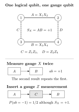
In the common $+1$ stabilizer sector, $A$ and $B$ represent the same gauge $X$. Measuring the anticommuting gauge operator $C$ between them destroys their outcome correlation. Both sequences leave the protected logical information intact when the gauge record is ignored; only the first product is a valid measurement of $S_X$.

For a general central stabilizer $S=G_1\cdots G_q$, a consecutive joint measurement of commuting factors gives its eigenvalue by multiplying their signed outcomes. Interleaving other gauge measurements requires a fresh analysis of the resulting instrument. Suchara, Bravyi, and Terhal (2011) develop conditions for valid syndrome inference from gauge sequences. Even a valid ideal instrument still needs a circuit that controls ancilla fault propagation and readout errors.

Gauge groups, logical operators, and distance

Let $\mathcal G$ be the physical Pauli gauge group, including scalar phases $\Phi=\langle iI\rangle$. For binary ranks write $\overline{\mathcal G}=\mathcal G/\Phi$. Multiplication modulo phase is abelian; the binary symplectic form retains the information about anticommutation of physical representatives. For a binary Pauli subspace $V$, let $V^\perp$ denote its symplectic orthogonal.

The stabilizer directions are

$$\overline{\mathcal S} =\overline{\mathcal G}\cap\overline{\mathcal G}^{\perp}.$$

Choose consistent Hermitian signs to define a signed stabilizer group $\mathcal S$ without $-I$. Its $+1$ sector is nonempty. The full group center also includes scalar phases, so it is $\Phi\mathcal S$, not the signed stabilizer group alone.

If the stabilizer rank is $s$ and the gauge algebra has $r$ independent anticommuting pairs, then

$$\begin{aligned} n&=s+k+r,\\ \dim\overline{\mathcal G}&=s+2r. \end{aligned}$$

The code is written $[[n,k,r,d]]$. Its encoded sector has dimension $2^{k+r}$; only $k$ qubits are protected. Count independent binary directions, not the number of measurements listed in a schedule.

A bare logical commutes with the whole gauge group and acts as $L\otimes I_G$. A dressed logical may act as $L\otimes g_G$. Multiplying by a gauge operator changes the gauge action without changing the protected action. The corresponding projective logical classes are

$$\begin{aligned} \mathcal L_{\rm bare} &=\overline{\mathcal G}^{\perp}/\overline{\mathcal S},\\ \mathcal L_{\rm dressed} &=\overline{\mathcal S}^{\perp}/\overline{\mathcal G}. \end{aligned}$$

Both have $2k$ binary dimensions. Their representatives need not have the same weights. For example, in the four-qubit code, multiplying $X_L=X_1X_3$ by $A$ gives $X_2X_3$. This is the same protected logical $X$, but it anticommutes with $C$ and is therefore dressed rather than bare.

The static Pauli distance minimizes over nontrivial dressed logicals:

$$d=\min_{v\in\overline{\mathcal S}^{\perp} \setminus\overline{\mathcal G}}\operatorname{wt}(v).$$

Poulin’s (2005) subsystem stabilizer formulation makes the recovery criterion especially direct. For every pair of correctable Pauli errors, $E_a^\dagger E_b$ must either anticommute with a stabilizer or belong to the gauge group. In the first case its compression to the encoded sector vanishes; in the second it acts only on $G$. A nontrivial dressed logical instead creates an ambiguity that recovery cannot resolve for all logical inputs.

Consequently, distance $d$ permits correction of all unknown errors on at most $\lfloor(d-1)/2\rfloor$ sites, or arbitrary errors on a known set of fewer than $d$ sites. These are different tasks. The four-qubit code has distance two: it detects every single-qubit Pauli and corrects any one known erasure, but cannot correct an arbitrary unknown single-qubit error. For instance, $X_1$ and $X_3$ differ by logical $X_L$ and have the same stabilizer syndrome.

Bacon–Shor rows and columns

Place qubits at sites $(i,j)$ of an $m\times n$ rectangle, with rows increasing downward. Following the convention above, the elementary gauges are horizontal $XX$ and vertical $ZZ$ bonds:

$$g^X_{i,j}=X_{i,j}X_{i,j+1},\qquad g^Z_{i,j}=Z_{i,j}Z_{i+1,j}.$$

Bacon (2006) introduced this lattice construction. Its stabilizers multiply all parallel bonds across one complete gap:

$$S^X_j=\prod_{i=1}^{m}g^X_{i,j},\qquad S^Z_i=\prod_{j=1}^{n}g^Z_{i,j}.$$

There are $n-1$ independent $X$ stabilizers and $m-1$ independent $Z$ stabilizers. Horizontal and vertical bond sets are separately independent, giving gauge rank $m(n-1)+n(m-1)$. Subtracting the center rank leaves twice the number of gauge qubits:

$$k=1,\qquad r=(m-1)(n-1).$$

A full column of $X$ and a full row of $Z$ are bare logicals. Each commutes with every gauge bond, and they anticommute with each other at their unique crossing. Moving a full column by multiplying an $X$ stabilizer changes its representative without changing its action on either encoded factor.

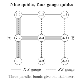
The $3\times3$ Bacon–Shor code has twelve weight-two gauge generators and four weight-six stabilizers. Multiplying the three horizontal bonds across a column gap gives one $X$ stabilizer. The highlighted column and row support a bare logical $X$ and $Z$. Four gauge qubits are encoded collective degrees of freedom, not four marked lattice sites.

A dressed logical $X$ must anticommute with a bare logical $Z$ on every row, since those row operators represent the same protected observable. It therefore has an $X$ or $Y$ on at least one site in every row and has weight at least $m$. Similarly, a dressed logical $Z$ has weight at least $n$. A logical $Y$ satisfies both requirements and cannot evade their lower bounds. The displayed pure strings attain them:

$$\begin{aligned} d_X&=m,\qquad d_Z=n,\\ d&=\min(m,n). \end{aligned}$$

Here the subscripts name the logical operator type, not the error type that an axis checks. The square family is $[[L^2,1,(L-1)^2,L]]$, giving $[[9,1,4,3]]$ at $L=3$.

Quantity	$3\times3$ block	$3\times5$ block
Physical qubits	9	15
Gauge qubits	4	8
Independent stabilizers	4	6
Gauge rank	12	22
$(d_X,d_Z)$	$(3,3)$	$(3,5)$

Decoding can ignore a site within a row

For $X$ errors, a $Z$ stabilizer compares the error parities of adjacent rows. Two $X$ errors in the same row multiply to a horizontal gauge string and are harmless to $L$. A single $X$ can therefore be corrected at any site in the correct row. For $Z$ errors the analogous equivalence is within a column. With independent Pauli components and perfect stabilizer measurements, decoding reduces to repetition decoding of row and column parities. Correlated components or nonuniform errors can change the most likely joint logical class.

The input to that decoder is a valid stabilizer syndrome, not an arbitrary product of gauge results. One simple ideal schedule measures all horizontal gauges in a commuting subround and then all vertical gauges. Noisy measurements require further processing and often repeated rounds; native parity measurements, ancilla circuits, routing, and leakage all affect performance. Decoders discusses inference from noisy records.

Growing distance is not enough for an accuracy threshold

Consider only independent $X$ errors of probability $p$ per site and perfect syndrome extraction on an odd square of side $L$. A row has odd error parity with probability

$$q_L=\frac{1-(1-2p)^L}{2}.$$

Majority decoding of the $L$ independent row parities fails with probability

$$P_X(L)=\sum_{j=(L+1)/2}^{L} \binom Lj q_L^j(1-q_L)^{L-j}.$$

At fixed $0<p<1/2$, $q_L$ approaches $1/2$ exponentially fast. The growing repetition block is then receiving almost completely random row bits, and $P_X(L)\to1/2$. The distance grows, but unrestricted growth of this particular block eventually hurts. Optimizing a finite rectangle for the noise can still produce strong protection; Napp and Preskill (2013) analyze that optimization. Aliferis and Cross (2007) instead obtain fault-tolerance results for a specified concatenated Bacon–Shor construction. Concatenation and increasing one square block are different code families.

Fixing a gauge and changing the code

Measuring an additional commuting gauge observable and choosing its sign reduces gauge freedom. In the four-qubit example, impose $C=+1$ alongside $S_X=S_Z=+1$. The remaining subspace encodes one qubit, with the same bare $X_L,Z_L$. If the measurement gives $C=-1$, applying $A$ flips that gauge sign without changing either logical observable. The procedure resets $G$ while preserving $L$.

More generally, choose a compatible commuting set of projective gauge directions $F$. Then

$$\begin{aligned} \overline{\mathcal S}'&=\langle\overline{\mathcal S},F\rangle,\\ \overline{\mathcal G}'&=\overline{\mathcal G}\cap F^\perp. \end{aligned}$$

Fixing $f$ new independent directions changes $s$ to $s+f$ and $r$ to $r-f$, while keeping $k$ fixed. Consistent measured signs and suitable gauge corrections specify the physical sector. Since $F$ lies in the original gauge algebra, bare logicals commute with it. Measuring a protected logical instead would change the task rather than fix a gauge.

Different choices can make different logical gates convenient. Vuillot and collaborators (2019) also formulate code deformation and lattice surgery in this language. The algebra explains the preserved logical information; Fault-Tolerant Gates and Lattice Surgery discuss the actual protocols. Endpoint distances alone do not establish the fault distance of a noisy transition.

Finally, low-weight gauge generators need not imply low-weight stabilizers. Square Bacon–Shor has weight-two gauges but weight-$2L$ center checks, so it does not meet the stabilizer-based definition of quantum LDPC codes. For two-dimensional Euclidean subsystem codes with bounded-range, bounded-density gauge generators, Bravyi (2011) proves $kd=O(n)$ and $d^2=O(n)$. If both gauge and stabilizer groups have spatially local generating sets, a stronger $kd^2=O(n)$ tradeoff applies under the stated hypotheses. Sparse long-range interactions do not satisfy these geometric assumptions.

Exercises

1. Conditional logical states

On the encoded factors, compare measuring $Z_G$ on $\rho_L\otimes|+\rangle\langle+|_G$ with measuring it on $(|0_L0_G\rangle+|1_L1_G\rangle)/\sqrt2$. Does a gauge measurement always preserve every conditional logical state?

Solution

For the product input, both outcomes have probability $1/2$ and leave $\rho_L$ unchanged. For the entangled input, the initial logical marginal is $I_L/2$, but selecting the positive outcome gives $|0_L\rangle$ and selecting the negative gives $|1_L\rangle$. Averaging the two returns $I_L/2$. Thus a gauge operation preserves the unconditional protected state; branch-by-branch preservation of an arbitrary original logical state additionally uses an uncorrelated input. No logical information can be signaled by an unrecorded local gauge measurement.

2. Recover the subsystem counts

A fifteen-qubit subsystem code has stabilizer rank six and gauge rank fourteen. Find $k$, $r$, and the encoded-sector dimension.

Solution

The noncentral gauge directions come in pairs: $2r=14-6=8$, so $r=4$. Then $k=15-6-4=5$ and the sector has dimension $2^{k+r}=512$. The number of protected states is $2^k=32$; the remaining factor is gauge freedom.

3. Write all four encoded basis states

Generate the four-qubit basis from $|0_L0_G\rangle$ using $X_L$ and $X_G$. Check the action of $Z_L$ and $Z_G$.

Solution

Using physical-bit order $1,2,3,4$,

$$\begin{aligned} |0_L0_G\rangle&=(|0000\rangle+|1111\rangle)/\sqrt2,\\ |0_L1_G\rangle&=(|1100\rangle+|0011\rangle)/\sqrt2,\\ |1_L0_G\rangle&=(|1010\rangle+|0101\rangle)/\sqrt2,\\ |1_L1_G\rangle&=(|0110\rangle+|1001\rangle)/\sqrt2. \end{aligned}$$

Each is a $+1$ eigenstate of $XXXX$ and $ZZZZ$. The parity of bits 1 and 2 gives the logical label; the parity of bits 1 and 3 gives the gauge label. Thus $Z_L$ and $Z_G$ act as the two independent computational-basis $Z$ operators. Equal coefficients ensure the $X$ operators flip their respective labels without additional phases.

4. A false syndrome with ideal measurements

Start in $\rho_L\otimes I_G/2$ in the four-qubit code. Find the joint outcome distributions for $A,B$ and for $A,C,B$.

Solution

For $A,B$, only $(a,b)=(+,+)$ and $(-,-)$ occur, each with probability $1/2$. For $A,C,B$, the three outcomes are independent fair signs, so each of the eight triples has probability $1/8$. Four triples have $ab=-1$. The true stabilizer remains $S_X=+1$ throughout. Inserting a gauge $Z$ measurement between two gauge $X$ measurements randomizes the result used in the proposed parity calculation.

5. Recovery modulo gauge

In the $3\times3$ code, compare errors $X_{2,1}$ and $X_{2,3}$. Then compare $X_{1,1}$ with $X_{2,1}X_{3,1}$.

Solution

The first pair differs by

$$X_{2,1}X_{2,3}=g^X_{2,1}g^X_{2,2},$$

so either representative corrects the protected information when either error occurs. The second pair differs by the full-column bare logical $X_{1,1}X_{2,1}X_{3,1}$. Their stabilizer syndromes also agree, but they have different logical actions. Correcting the two-site error as if it were the one-site error produces a logical failure. Equal syndrome is therefore weaker than equivalence modulo gauge.

6. A rectangular block under independent bit flips

For a $3\times5$ block with independent physical $X$ error probability $p$, derive the logical $X$ failure probability with perfect syndrome measurements and majority decoding. Obtain its leading small-$p$ behavior.

Solution

Each row contains five sites. The generating function for its parity gives $q=(1-(1-2p)^5)/2=5p+O(p^2)$. At least two of three row parities must be odd for majority decoding to fail:

$$\begin{aligned} P_X&=3q^2(1-q)+q^3\\ &=3q^2-2q^3\\ &=75p^2+O(p^3). \end{aligned}$$

The distance is still $d_X=3$, but the coefficient counts more ways to make two odd rows than in a $3\times3$ block, whose coefficient is $27$. Lengthening rows improves the logical-$Z$ distance while making this logical-$X$ channel worse at leading order. Geometry must be chosen for the noise, not from the smaller distance alone.

7. Fix a gauge without measuring the logical qubit

In the four-qubit code measure $C$ and, on a negative outcome, apply $A$. What are the final stabilizers, logical operators, and distance? What happens to an arbitrary initial gauge state?

Solution

The final independent stabilizers are $S_X,S_Z,C$, all with positive sign. There is one logical qubit and no gauge qubit. The bare $X_L=X_1X_3$ and $Z_L=Z_1Z_2$ still commute with these checks and anticommute with each other. Every single-site nonidentity Pauli anticommutes with $S_X$ or $S_Z$, while the displayed weight-two logicals survive, so the subspace distance is two.

On the gauge factor the two corrected Kraus operators are $|0\rangle\langle0|$ and $|0\rangle\langle1|$. Ignoring the measurement result resets any gauge state to $|0_G\rangle$. For an initially correlated state the complete map is $\rho_{LG}\mapsto\rho_L\otimes|0\rangle\langle0|_G$, preserving the original logical marginal.

8. Apply the geometric hypothesis

Could a two-dimensional Euclidean family with bounded-range, bounded-density gauge generators have $k=\Theta(n^{2/3})$ and $d=\Theta(n^{1/2})$? Would bounded check weight alone give the same conclusion?

Solution

The proposed product is $kd=\Theta(n^{7/6})$, violating $kd=O(n)$ under the stated geometric hypotheses. Bounded weight alone does not bound the length of an interaction or the density of physical sites in the plane, so the theorem does not rule out an abstract nongeometric family with those exponents. Counting check support and specifying spatial locality answer different questions.

References

• P. Aliferis and A. W. Cross, “Subsystem fault tolerance with the Bacon–Shor code,” Physical Review Letters 98, 220502 (2007), doi:10.1103/PhysRevLett.98.220502, arXiv:quant-ph/0610063.
• D. Bacon, “Operator quantum error-correcting subsystems for self-correcting quantum memories,” Physical Review A 73, 012340 (2006), doi:10.1103/PhysRevA.73.012340, arXiv:quant-ph/0506023.
• S. Bravyi, “Subsystem codes with spatially local generators,” Physical Review A 83, 012320 (2011), doi:10.1103/PhysRevA.83.012320, arXiv:1008.1029.
• D. W. Kribs, R. Laflamme, D. Poulin, and M. Lesosky, “Operator quantum error correction,” Quantum Information and Computation 6, 382–399 (2006), doi:10.26421/QIC6.4-5-6, arXiv:quant-ph/0504189.
• J. Napp and J. Preskill, “Optimal Bacon–Shor codes,” Quantum Information and Computation 13, 490–510 (2013), doi:10.26421/QIC13.5-6-9, arXiv:1209.0794.
• D. Poulin, “Stabilizer formalism for operator quantum error correction,” Physical Review Letters 95, 230504 (2005), doi:10.1103/PhysRevLett.95.230504, arXiv:quant-ph/0508131.
• M. Suchara, S. Bravyi, and B. M. Terhal, “Constructions and noise threshold of topological subsystem codes,” Journal of Physics A: Mathematical and Theoretical 44, 155301 (2011), doi:10.1088/1751-8113/44/15/155301, arXiv:1012.0425.
• C. Vuillot, L. Lao, B. Criger, C. García Almudéver, K. Bertels, and B. M. Terhal, “Code deformation and lattice surgery are gauge fixing,” New Journal of Physics 21, 033028 (2019), doi:10.1088/1367-2630/ab0199, arXiv:1810.10037.