Logical Benchmarking

A logical benchmark measures how well encoded information survives a specified memory interval, gate or circuit. It includes the syndrome-processing and recovery rule used to interpret the output. A detection event, a physical gate fidelity and a logical failure probability describe different things; none can replace the others without a model.

The first task is to define what the experiment observes. A final logical measurement usually reveals an endpoint error, not every logical fault that occurred along the way. Discarding flagged trials changes the sampled ensemble. Comparing code distances tests suppression, while comparing against an unencoded reference tests break-even. Keeping these distinctions explicit makes the measured number useful.

Required background. Quantum error correction explains correctability; stabilizers define logical operators and syndromes; decoders explain how a syndrome record becomes a logical decision.

Measure an encoded operation on a logical space

For an unconditional experiment, a schematic decoded channel is

$$\mathcal L=\mathcal D\circ\mathcal R \circ\mathcal N\circ\mathcal E.$$

Here $\mathcal E$ encodes the input, $\mathcal N$ implements the noisy protected operation, $\mathcal R$ includes recovery or frame interpretation, and $\mathcal D$ returns a logical output. An actual protocol may interleave these steps and use a classical syndrome register. The expression defines the input and output spaces; it is not a prescription to physically decode the qubit before every measurement.

If the endpoint is destructive readout, its measured object can be a quantum-to-classical channel rather than a complete surviving quantum state. If leakage or rejection remains possible, include those outputs explicitly. Projecting onto the code space and renormalizing is not an unconditional decoding channel.

A memory experiment prepares known encoded states, runs several correction rounds, and measures logical observables. Testing only $|0_L\rangle$ cannot reveal a logical $Z$ error. Preparing the six Pauli eigenstates and measuring their corresponding survival probabilities probes all three axes, but those survival measurements alone are not full process tomography: they do not determine every off-diagonal transfer-matrix element.

For a Pauli logical channel,

$$\mathcal L(\rho)=\sum_{P\in\{I,X,Y,Z\}}p_P P\rho P,$$

the axis-dependent error probabilities are

$$\begin{aligned} e_X&=p_Y+p_Z,\\ e_Y&=p_X+p_Z,\\ e_Z&=p_X+p_Y. \end{aligned}$$

Here $e_Z$ means a wrong outcome when a $Z$ eigenstate is prepared and read in the $Z$ basis. It is different from the probability $p_Z$ of a logical $Z$ operator. This notation prevents a common ambiguity in a reported “$Z$ error rate.” The total nonidentity Pauli probability is

$$p_{\mathrm{Pauli}}= \frac{e_X+e_Y+e_Z}{2}.$$

For example, $(p_I,p_X,p_Y,p_Z)=(0.94,0.01,0.02,0.03)$ gives:

Prepared and measured axis	Wrong-outcome probability
$X$	$0.05$
$Y$	$0.04$
$Z$	$0.03$

The total Pauli probability is $0.06$, while average state infidelity is $0.04$. These are compatible summaries of the same channel, not competing estimates of one number. Coherent logical rotations need more information; hardware metrics explains their relation to worst-case error.

Endpoint error and error per round are different

Suppose a chosen logical binary observable flips independently with probability $e$ each round. Let $N_r$ count flips in $r$ rounds. The final outcome is wrong only when $N_r$ is odd. Since each round multiplies its sign by $-1$ with probability $e$,

$$C(r)=\mathbb E[(-1)^{N_r}]=(1-2e)^r.$$

Thus

$$P_{\mathrm{wrong}}(r)=\frac{1-(1-2e)^r}{2}.$$

This is not the probability that at least one flip occurred,

$$P(N_r\geq1)=1-(1-e)^r.$$

The latter approaches one, while the endpoint error approaches one half. For $e=0.05$ and $r=20$, they are approximately 0.642 and 0.439 respectively. Two flips can restore the final bit, so counting endpoint failures and dividing by the total number of rounds is generally not an estimator of the per-round flip probability.

At small $re$, both probabilities are approximately $re$. That approximation is useful only before saturation and within the independent-flip model. In a simulation, access to the sampled error history may reveal a latent logical fault that the laboratory endpoint measurement cannot identify.

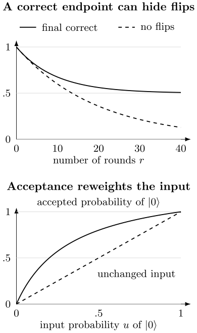
Top: independent flips with probability $0.05$ per round. The final bit can be correct even when flips occurred. Bottom: the accepted filter $K_A=\operatorname{diag}(1,1/2)$ changes a diagonal input’s zero-state probability from $u$ to $u/[u+(1-u)/4]$. The dashed diagonal would preserve that probability. Conditioning must be included when interpreting accepted outputs.

Fit a decay only when its model fits

Stable preparation and readout errors can motivate a survival fit

$$P_{\mathrm{correct}}(r)=A+B\lambda^r.$$

For the independent binary-flip interpretation, $\lambda=1-2e$. The fitted $A$ and $B$ describe boundary effects; they do not automatically remove arbitrary state-preparation or measurement errors. Several decay modes, leakage, coherent oscillations and drift can invalidate the form.

Use several round counts, including short controls and longer durations with measurable decay. Inspect residuals and stability when the fitting interval changes. Very short data may be dominated by boundaries; very long data may be nearly random and insensitive to the desired rate.

For $0\leq e<1/2$ and cycle time $\tau$, an equivalent continuous-time Poisson flip rate is

$$\Gamma=-\frac{\ln(1-2e)}{2\tau}.$$

It reproduces $C(t)=e^{-2\Gamma t}$ at the sampled times. This is a model-dependent conversion, not an assertion that the physical process is literally Poisson. For small $e$, $\Gamma\approx e/\tau$. Report the cycle duration when comparing rates.

Postselection produces an instrument

Let $\mathcal J_A$ and $\mathcal J_R$ be the accepted and rejected completely positive branches of an experiment. Their sum is trace preserving when every outcome is included. The acceptance probability is

$$a(\rho)=\operatorname{Tr}\mathcal J_A(\rho),$$

and the accepted state is

$$\rho_A=\frac{\mathcal J_A(\rho)}{a(\rho)}$$

when $a(\rho)>0$. If acceptance depends on $\rho$, this normalized transformation is generally nonlinear. Calling it a single trace-preserving logical channel would lose that dependence. The unnormalized branch and the full flagged output remain linear physical descriptions.

An exact example uses

$$\begin{aligned} K_A&=\begin{pmatrix}1&0\\0&1/2\end{pmatrix},\\ \mathcal J_A(\rho)&=K_A\rho K_A^\dagger. \end{aligned}$$

The complementary rejected Kraus operator is $K_R=\operatorname{diag}(0,\sqrt3/2)$. Both basis states are unchanged after acceptance, but their acceptance probabilities are 1 and $1/4$. The input $I/2$ is accepted with probability $5/8$ and becomes $\operatorname{diag}(4/5,1/5)$. It is not the equal mixture of the separately normalized basis outputs.

For a specified benchmark ensemble, let $a$ be its average acceptance and $p_{L|A}$ its accepted wrong-outcome probability. Then

$$\begin{aligned} P_{\mathrm{good}}&=a(1-p_{L|A}),\\ P_{\mathrm{bad}}&=ap_{L|A},\\ P_{\mathrm{reject}}&=1-a. \end{aligned}$$

Report all three categories, or equivalently $a$ and $p_{L|A}$. A low conditional error may be valuable for a heralded primitive. It does not describe delivery on every attempt. If acceptance differs between input states, also report that variation instead of averaging it away.

Being outside a stabilizer code space is not automatically physical leakage: an ordinary correctable Pauli error produces a nontrivial syndrome. Distinguish computational-subspace leakage, a flagged erasure, a correctable syndrome and a residual logical error. They have different meanings for recovery and selection.

Logical gates and randomized sequences

A gate benchmark must include the preparation, correction rounds, ancillas, decoded measurement results and conditional operations that its intended use requires. A comparison with an equal-duration logical identity helps separate storage error from the gate’s added error. Controlled fault injection tests error containment, but testing a few injected faults does not prove that every allowed fault set is harmless.

Logical randomized benchmarking samples logical Clifford sequences, appends the ideal inverse, and measures survival. Combes and collaborators propose a protocol operating directly at the encoded level. In the usual gate-independent, stationary Markovian logical-noise model, Clifford averaging yields

$$P_{\mathrm{surv}}(m)=A+B\alpha_L^m.$$

For a logical space of dimension $D_L$, the associated average infidelity is

$$r_L=\frac{D_L-1}{D_L}(1-\alpha_L).$$

This is per sampled, implemented logical Clifford. It is not automatically per physical gate, per correction round or the worst logical gate. Its conversion follows the assumptions of standard randomized benchmarking; the canonical explanation derives the twirl and fitting model.

Physical noise being stationary does not guarantee a memoryless logical process. Syndrome degrees of freedom, incomplete resets and decoder state can retain information between logical operations. Ceasura and collaborators construct nonexponential logical-RB behavior with gate- and time-independent physical noise. More general representation-based treatments can have several decay modes; see Helsen and collaborators.

An oscillation or multiexponential curve therefore deserves diagnosis, not a forced one-rate summary. Leakage-sensitive measurements, syndrome-reset variations and sequence-level residuals can distinguish hypotheses. A nonexponential curve alone does not identify a unique cause: a mixture of two stationary populations already gives two exponentials.

Interleaving a target gadget inherits the assumptions and uncertainty of the reference protocol. Cycle benchmarking addresses parallel layers. Non-Clifford injection additionally couples the delivered gate to resource-state quality, acceptance and classical reaction time. A memory benchmark cannot establish those operations’ performance.

Uncertainty depends on independent repetitions

If $n$ independent identical trials yield $k$ wrong outcomes, the binomial likelihood is proportional to $p^k(1-p)^{n-k}$ and the estimate is $k/n$. Here one trial might be a complete fixed-length memory experiment. Calling all its internal rounds independent trials changes the likelihood without justification.

For zero observed failures, the probability of that observation at error rate $p$ is $(1-p)^n$. Equating this probability to $\alpha$ gives the one-sided upper confidence limit

$$p_U=1-\alpha^{1/n}.$$

At 95% confidence and large $n$, this is approximately $3/n$. Zero failures in 500,000 independent trials give about $6.0\times10^{-6}$, not a demonstrated zero rate.

If shots share drift or a common burst, use the sampling clusters that are independent under the model. Five thousand independent blocks of 100 perfectly correlated shots contain 5,000 independent Bernoulli outcomes, not 500,000. The corresponding zero-failure limit is about $6.0\times10^{-4}$. Actual partial correlations require a suitable joint or clustered model; an arbitrary “effective sample size” is not a substitute for one.

For nonzero counts, use intervals appropriate to the likelihood and probability boundary rather than symmetric normal errors near zero. Randomized sequences create an additional sampling level: repeating one sequence many times reduces its shot noise but does not sample other sequences. Preserve the hierarchy of sequences, shots and chronological blocks when fitting or resampling.

Choose stopping and selection rules before examining the final evaluation data. Tuning decoder weights or acceptance cuts on those data can bias the reported improvement. Time-ordered holdout blocks are particularly useful when calibration drifts. Rare-event simulations and extrapolations can extend a tested model’s predictions, but their uncertainty and model dependence must remain distinct from directly observed frequencies.

Suppression and break-even answer different questions

For matched tasks at distances $d$ and $d+2$, define

$$\Lambda=\frac{p_L(d)}{p_L(d+2)}.$$

Values above one mean the larger tested code performs better for this metric. Match the state ensemble, elapsed-time or round convention, physical operating conditions, decoder information and acceptance rule. A better-selected hardware subset or more informative decoder can improve performance without the improvement being due solely to distance.

For independent estimates with small relative uncertainty, the delta method gives

$$\operatorname{Var}(\ln\widehat\Lambda) \approx\frac{\operatorname{Var}(\widehat p_d)}{p_d^2} +\frac{\operatorname{Var}(\widehat p_{d+2})}{p_{d+2}^2}.$$

Paired estimates require a covariance term, $-2\operatorname{Cov}(\widehat p_d,\widehat p_{d+2})/(p_dp_{d+2})$. Near zero failures, this approximation is unsuitable; use a joint likelihood or a justified interval respecting the boundary.

Break-even instead compares a logical implementation with a specified reference:

$$G=\frac{p_{\mathrm{ref}}}{p_L}.$$

The reference might be the best physical carrier, an uncorrected encoded memory, or a physical implementation of the same gate. Align task, time and acceptance. A larger code can suppress errors relative to a smaller code while still being worse than that reference. Conversely, a fixed code may beat a physical reference without establishing asymptotic scaling. The threshold theorem explains why finite comparisons do not prove an infinite-family result.

The decoder is part of the operation being compared. Offline access to later syndrome rounds is useful for retrospective inference, but an adaptive gate may need its decision before those rounds exist. Evaluate accuracy under the observations and deadlines that the intended computation supplies. Keep decoder throughput, latency tails, trial duration, acceptance and physical occupancy alongside reliability. These quantities become inputs to resource estimation.

Exercises

1. Reconstruct a Pauli error distribution

Measured axis errors are $e_X=0.05$, $e_Y=0.04$, $e_Z=0.03$. Under the Pauli-channel assumption, recover the four probabilities and the average infidelity.

Solution

Solving the three linear equations gives

$$p_X=\frac{e_Y+e_Z-e_X}{2}=0.01.$$

Similarly $p_Y=0.02$, $p_Z=0.03$ and $p_I=0.94$. Each nonidentity Pauli has average state infidelity $2/3$, so the channel’s average infidelity is $(2/3)(0.06)=0.04$. Negative reconstructed probabilities are incompatible with a physical Pauli channel at the point-estimate level. Examine sampling uncertainty, preparation/readout errors and inconsistent conditions; coherence alone need not produce negative values.

2. Count odd flips rather than any flip

Independent logical flips have probability $e=0.05$ per round. Compute the endpoint error and probability of at least one flip after 20 rounds. Does dividing endpoint error by 20 recover $e$?

Solution

The endpoint error is $(1-0.9^{20})/2\approx0.4392$. The probability of at least one flip is $1-0.95^{20}\approx0.6415$. Endpoint error divided by 20 is about 0.0220, well below 0.05. Even flip counts restore the measured bit. Recovering $e$ requires the model-dependent decay relation, not that division.

3. Compare per-round and per-time performance

Memory A has binary flip probability $4\times10^{-4}$ per $1\,\mu\mathrm{s}$ cycle; B has $6\times10^{-4}$ per $4\,\mu\mathrm{s}$ cycle. Compare their independent-flip models at equal cycle count and equal elapsed time.

Solution

A is better per cycle. At equal time, use

$$\Gamma_A\approx400\,\mathrm{s}^{-1}, \qquad\Gamma_B\approx150\,\mathrm{s}^{-1}.$$

B then has less parity decay at the same elapsed time. The exact logarithmic rates are about $400.16\,\mathrm{s}^{-1}$ and $150.09\,\mathrm{s}^{-1}$. This comparison concerns storage, not the speed of a logical gate that uses those cycles.

4. Test linearity after acceptance

Use $K_A=\operatorname{diag}(1,1/2)$. Compare filtering $I/2$ and normalizing with filtering $|0\rangle$ and $|1\rangle$ separately, normalizing each, and mixing them equally. Explain the difference.

Solution

The first procedure gives

$$K_A(I/2)K_A^\dagger =\operatorname{diag}(1/2,1/8),$$

whose trace is $5/8$. Normalizing gives $\operatorname{diag}(4/5,1/5)$. Each separately accepted basis state is unchanged, so their equal mixture is $I/2$. The accepted ensemble reweights the inputs by their unequal success probabilities. The unnormalized branch remains linear; normalization causes the discrepancy.

5. Count independent blocks

No failures occur in 500,000 shots arranged in 5,000 independent blocks. Within each block the 100 outcomes are identical. Find the one-sided 95% upper limit on the marginal failure probability.

Solution

The probability of zero failures is $(1-p)^{5000}$, so

$$p_U=1-0.05^{1/5000} \approx5.99\times10^{-4}.$$

Using 500,000 independent shots instead would give $5.99\times10^{-6}$, understating the limit by about a factor of 100. This exact example illustrates why a correlated sample cannot simply be treated as binomial at the shot level.

6. Quantify suppression without break-even

Two independent million-trial memory experiments give 900 and 300 errors. A matched physical reference has known error probability $2\times10^{-4}$. Estimate suppression, an approximate 95% interval for its ratio, and break-even gain for the better code.

Solution

The point estimate is $\widehat\Lambda=3$. Its approximate log standard error is

$$\begin{aligned} \sigma_{\ln\Lambda} &=\sqrt{\frac{1-0.0009}{900} +\frac{1-0.0003}{300}}\\ &\approx0.0667. \end{aligned}$$

The interval $3\exp(\pm1.96\sigma_{\ln\Lambda})$ is approximately $[2.63,3.42]$. It supports suppression in this finite comparison. The break-even gain is $2/3<1$, so the better code still underperforms the stated reference. An estimated reference rate would need its own uncertainty.

7. A mixture does not have one decay rate

Half the trials have independent flip rate 0.001 per round; half have rate 0.01, with that rate fixed throughout each trial. Find the averaged correlation. Compare effective per-round errors inferred separately from rounds 0–100 and 100–200.

Solution

The correlation is

$$C(r)=\frac12(0.998)^r+\frac12(0.98)^r.$$

It gives $C(100)\approx0.47559$ and $C(200)\approx0.34382$. Fitting each interval by one exponential gives the factors

$$\begin{aligned} \lambda_{0:100}&=C(100)^{1/100},\\ \lambda_{100:200}&=[C(200)/C(100)]^{1/100}. \end{aligned}$$

Using $e=(1-\lambda)/2$ gives inferred errors approximately 0.00370 and 0.00162 respectively. The faster-decaying population contributes progressively less to the remaining correlation. The changing fitted rate does not require either population’s physical rate to vary within a trial.

8. Keep acceptance beside correctness

A known-output benchmark accepts 20% of trials and has wrong-output probability $10^{-3}$ among accepted trials. Each attempt takes 5 ms. Compute its correct accepted output rate and mean attempts per accepted output under independent stationary trials.

Solution

The ensemble rate is

$$R_{\mathrm{good}}= \frac{0.2(1-10^{-3})}{0.005\,\mathrm{s}} =39.96\,\mathrm{s}^{-1}.$$

The mean attempts per accepted output is $1/0.2=5$. The rate counts correct outcomes relative to the benchmark’s known answer; it does not supply a general procedure to recognize errors in an unknown quantum output. Acceptance is visible, correctness need not be.

References

• A. Ceasura, P. Iyer, J. J. Wallman and H. Pashayan, “Non-exponential behaviour in logical randomized benchmarking,” arXiv:2212.05488 (2022), arXiv.
• J. Combes, C. Granade, C. Ferrie and S. T. Flammia, “Logical randomized benchmarking,” arXiv:1702.03688 (2017), arXiv.
• J. Helsen, I. Roth, E. Onorati, A. H. Werner and J. Eisert, “General framework for randomized benchmarking,” PRX Quantum 3, 020357 (2022), doi:10.1103/PRXQuantum.3.020357.
• E. Magesan, J. M. Gambetta and J. Emerson, “Scalable and robust randomized benchmarking of quantum processes,” Physical Review Letters 106, 180504 (2011), doi:10.1103/PhysRevLett.106.180504, arXiv:1009.3639.