Magic State Distillation

Magic state distillation trades several imperfect nonstabilizer ancillas for fewer, cleaner ones using Clifford operations, Pauli measurements and postselection. The accepted states can then implement non-Clifford gates on data. The central tradeoff is between output quality, acceptance probability and the work needed to obtain each accepted output.

We will derive a $T$-gate injection, explain the noise assumptions behind a scalar distillation map, and work through the 15-to-1 protocol. Its familiar $35p^3$ law is a small-error result for independent inputs and ideal Clifford processing. Correlations, faulty checks and finite output supply require additional analysis.

Required background. Stabilizer Formalism supplies Pauli checks and logical operators; Fault-Tolerant Gates explains protected gadgets; Universal Gate Sets explains why adding $T$ to Clifford operations gives universality.

The resource state for a T gate

Use the convention

$$T=\operatorname{diag}(1,e^{i\pi/4}),\qquad S=T^2,$$

and define

$$|T\rangle=T|+\rangle =\frac{|0\rangle+e^{i\pi/4}|1\rangle}{\sqrt2}.$$

Its Bloch vector is $(1,1,0)/\sqrt2$, outside the octahedron of single-qubit stabilizer mixtures. Clifford operations and Pauli measurements alone cannot create it from stabilizer inputs. It is consequently a resource relative to that restricted set of operations; Resource Theories explains this general idea.

Names vary across the literature. The state called $|T\rangle$ here is Clifford-equivalent to a Hadamard eigenstate. Bravyi and Kitaev (2005) call this family H-type; their T-type states point along a different Bloch-sphere direction. Stating the vector prevents confusion between their five-qubit protocol and the 15-to-1 protocol considered below.

Magic-state consumption is useful when logical Clifford operations are easier to protect than the desired non-Clifford gate. A code with a transversal $T$ gate can have a different expensive operation. Distillation is therefore an architectural option, not a universal requirement for every fault-tolerant design.

Injection with one ancilla and feedforward

Prepare data $|\psi\rangle=a|0\rangle+b|1\rangle$ and an ancilla $|T\rangle$. Apply CNOT with data as control and ancilla as target, then measure the ancilla in the computational basis. The unnormalized data outputs are

$$\begin{aligned} m=0:&\quad \frac{1}{\sqrt2}T|\psi\rangle,\\ m=1:&\quad \frac{e^{i\pi/4}}{\sqrt2}T^\dagger|\psi\rangle. \end{aligned}$$

Both outcomes have probability $1/2$. For outcome one, apply $S$, since $ST^\dagger=T$. The corrected output is always $T|\psi\rangle$, up to a branch phase.

The state has supplied the non-Clifford part; the remaining circuit uses Clifford operations and a Pauli measurement. Fault-tolerant injection still requires protected CNOT, readout and classical decisions. A correction can sometimes be tracked in a Clifford frame, but later operations must be adapted to that frame. A bad ancilla can inject an error directly into the data.

A noise model that can be distilled

Let $|T_\perp\rangle=Z|T\rangle$. These states are orthogonal eigenvectors of the Hermitian Clifford operator

$$W=(X+Y)/\sqrt2.$$

The eigenvalues are $+1$ and $-1$, respectively. Applying $I$ or $W$ with equal probability and discarding the random choice dephases a qubit in this basis:

$$\mathcal T_W(\rho)=\tfrac12(\rho+W\rho W).$$

The resulting state is

$$\rho_p=(1-p)|T\rangle\langle T| +p|T_\perp\rangle\langle T_\perp|,$$

where $p=\langle T_\perp|\rho|T_\perp\rangle$. This twirl preserves the target-state fidelity while removing coherence between the two basis states. In the injection circuit above, this diagonal resource produces the ideal $T$ gate followed by a stochastic $Z$ error of probability $p$.

Independent twirling of many inputs makes their joint state diagonal in the product basis, but it does not make their classical error variables independent. A shared preparation fault survives as a correlation. Leakage outside the qubit space and faults during the twirl are also outside this ideal two-state model.

For $0\le p\le1/2$, the Bloch vector of $\rho_p$ is $(1-2p)(1,1,0)/\sqrt2$. It becomes a stabilizer mixture when

$$p\ge p_{\rm stab}=\frac{1-1/\sqrt2}{2} \simeq0.14645.$$

This boundary is a property of the state family and free operations. It need not equal the threshold of a particular distillation protocol. Having a nonstabilizer state does not imply that every chosen protocol improves it.

Acceptance and conditional output quality

A protocol’s accepted branch is a completely positive, trace-nonincreasing map $\mathcal D_{\rm acc}$. For a joint input $\rho_n$, define

$$\begin{aligned} A(\rho_n)&=\operatorname{Tr}\mathcal D_{\rm acc}(\rho_n),\\ \rho_{\rm out}&=\mathcal D_{\rm acc}(\rho_n)/A(\rho_n). \end{aligned}$$

The first quantity is the acceptance probability. The second is the state conditioned on acceptance, provided $A>0$. Normalization makes this conditional transformation nonlinear as a function of the input; the unnormalized accepted map remains linear.

For identical independent diagonal inputs $\rho_p^{\otimes n}$, a one-output protocol may reduce to functions $A(p)$ and $p_{\rm out}=f(p)$. Improvement means $f(p)<p$, not merely that an accepted state was produced. With independent retries, the expected input-state consumption per accepted output is $n/A(p)$. This does not count protected gates, storage or routing.

Bravyi and Kitaev (2005) establish distillation using noisy ancillas and ideal stabilizer operations. In a hardware implementation, the stabilizer operations are themselves encoded and imperfect. It is useful to solve the ideal map first, then identify which additional errors enter the actual accepted ensemble.

Why fifteen inputs give cubic suppression

The 15-to-1 construction uses the phase structure of the punctured quantum Reed–Muller code. After the ideal Clifford processing is accounted for, the diagonal input errors can be represented by fifteen binary variables $e_j$. A one denotes a $Z$ error on that resource.

Let $H$ be the $4\times15$ binary matrix whose columns are the fifteen distinct nonzero four-bit vectors, ordered by the integers $1,\ldots,15$. The run accepts when

$$He=0\pmod2.$$

For an accepted pattern, the output error bit is the total parity

$$\ell(e)=\sum_{j=1}^{15}e_j\pmod2.$$

These rules describe the input-error propagation in the ideal distillation circuit; simply measuring four ordinary $X$ checks directly on fifteen unprocessed magic states is not the same protocol. Encoding, the phase-gate pattern and Clifford corrections establish this classical description. Bravyi and Haah (2012) explain its relation to triorthogonal constructions.

Every single error produces a nonzero column syndrome. Every pair produces the XOR of two distinct columns, also nonzero. Hence all weight-one and weight-two input errors are rejected.

For a triple, the syndrome vanishes precisely when its columns obey $u\oplus v\oplus w=0$. Any two distinct nonzero columns determine the third, and each triple is counted three times by its pairs. There are therefore

$$\frac{\binom{15}{2}}3=35$$

accepted triples. All have odd parity and hence cause an output error. For independent errors of small probability $p$, each such pattern has probability $p^3(1-p)^{12}$. Their leading contribution is $35p^3$; acceptance tends to one as $p\to0$.

The exact map

Write $x=1-2p$. Every nonzero binary combination of the four rows of $H$ has weight eight. Averaging the corresponding parity signs gives

$$A(p)=\frac{1+15x^8}{16}.$$

To separate accepted even and odd patterns, define their signed difference

$$C(p)=\frac{x^{15}+15x^7}{16}.$$

Then their total is $A$ and their difference is $C$, so the conditional odd probability is

$$f(p)=\frac{A(p)-C(p)}{2A(p)}.$$

This also gives the commonly written rational expression

$$f(p)=\frac{1-15x^7+15x^8-x^{15}} {2(1+15x^8)}.$$

Near zero, $A(p)=1-15p+105p^2+O(p^3)$ and $f(p)=35p^3+O(p^4)$. Subtracting nearly equal numbers in $A-C$ is numerically unstable at extremely small $p$. One can instead sum the nonnegative probabilities of accepted odd-weight patterns, or use higher-precision arithmetic.

The useful nonzero fixed point is $p_*\simeq0.14148$. Below it, the ideal map improves these inputs; immediately above it, it worsens them. This is a 15-to-1 protocol threshold, assuming independent diagonal inputs and perfect Clifford processing. It is smaller than $p_{\rm stab}$ and is unrelated to a physical surface-code threshold.

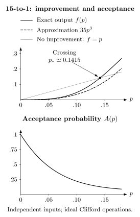
Top: improvement occurs where the exact output curve lies below the identity line. The crossing is near $p=0.1415$. The cubic approximation is useful near zero but misses the crossing quantitatively. Bottom: acceptance decreases as the inputs become noisier, so the raw-state cost rises even before improvement stops. Both panels assume the ideal independent-input model.

Input error $p$	Acceptance $A$	Output error $f$
0.001	0.9851	$3.51\times10^{-8}$
0.01	0.8601	$3.61\times10^{-5}$
0.10	0.2198	0.0477

At $p=0.001$, one accepted output consumes about $15.23$ raw states on average. At $p=0.10$, it consumes about $68.25$. A clean conditional output and a high yield are separate desirable properties.

Correlations and imperfect checks

The cubic law depends on probabilities of complete patterns. Consider a batch with no error with probability $1-q$, and with probability $q$ choose uniformly one of the 35 accepted triples. Every batch accepts. Every faulty batch produces a logical output error, so $p_{\rm out}=q$.

Each input belongs to seven of the triples. All fifteen marginals are therefore identical, with $p=q/5$. An independent-input model with those same marginals would predict about $35(q/5)^3$, while the actual output error is $q=5p$. Even equal input fidelities and ideal twirling do not establish independent inputs.

Faulty Clifford checks introduce another issue: their error contribution must be evaluated conditioned on acceptance. If a harmful circuit event has unconditional probability at most $q$, then

$$\Pr(\text{harmful}\mid\text{accept}) \le\frac{q}{\Pr(\text{accept})}.$$

Thus an unconditional circuit-error estimate cannot simply be added to the ideal conditional output error without accounting for the acceptance event. A rare fault that both damages the output and forces acceptance is particularly important. Exercise 5 gives an exact example.

For a stage model $p_{\ell}\lesssim f(p_{\ell-1})+\delta_{\ell}$, the term $\delta_{\ell}$ must be a justified bound in the accepted ensemble, with any acceptance changes included. Once that term dominates, adding another ideal distillation stage without improving its protected implementation will not achieve the ideal recurrence’s tiny output error.

The same conditioning matters for catalysts and multiple outputs. A persistent catalyst fault can correlate outputs from many rounds. O’Gorman and Campbell (2017) analyze correlated outputs in factory estimates; Gidney and Fowler (2019) discuss a catalyzed conversion from CCZ resources to two $T$ states. Returning a catalyst does not mean its errors are reset.

Recursive purification and other resource choices

If each new level receives genuinely independent outputs from separate lower-level attempts, the ideal recurrence is $p_\ell=f(p_{\ell-1})$. At $p_0=10^{-3}$, two ideal 15-to-1 levels give approximately

$$\begin{aligned} p_1&=3.51\times10^{-8},\\ p_2&=1.51\times10^{-21}. \end{aligned}$$

The second number describes the ideal map, not a predicted hardware error. Even a small conditional circuit contribution can dominate it.

For independent retries and one output per block, expected raw consumption obeys

$$C_\ell=C_{\ell-1}\frac{15}{A(p_{\ell-1})}, \qquad C_0=1.$$

Two such levels at this input error consume about $228.4$ raw states per accepted output. The number exceeds $15^2=225$ because rejected attempts also consume inputs. Finite buffers, shared drift and batch-dependent acceptance can require a more detailed model.

Several alternatives change this tradeoff. Meier, Eastin, and Knill (2013) use ten inputs to produce two improved Hadamard-type states. These are Clifford-equivalent to our resource, but their protocol has different checks, suppression and yield. Bravyi–Haah blocks can produce several outputs, with correlations that must be retained when those outputs feed another stage.

In the latter construction, a binary matrix is triorthogonal when each pair and each triple of distinct rows have even overlap. Odd-weight rows identify logical $X$ operators; even-weight rows supply $X$ stabilizers. The overlap conditions arrange a transversal phase operation, with possible Clifford corrections, to act appropriately on the encoded information. They do not by themselves give an output-error rate: the undetected patterns and their probabilities still have to be counted.

A workload dominated by Toffoli gates may benefit from a direct CCZ resource instead of compiling every operation into separate $T$ injections. Code switching and pieceable gates offer other routes, as explained in Fault-Tolerant Gates. Current experimental milestones and newer preparation proposals are discussed in Fault-Tolerant Quantum Computing Frontier; the ideal maps here establish neither sustained hardware throughput nor an experimental error floor.

Supplying resources when the algorithm needs them

A factory repeatedly prepares and checks resources, then stores and delivers accepted outputs. If $F$ independent units each attempt a $k$-output batch every $\tau$, with acceptance probability $A$, the nominal mean supply is

$$R=\frac{FkA}{\tau}.$$

Mean supply exceeding mean demand does not guarantee that every requested resource arrives on time. Rejections are random, batches can be correlated, routes can be occupied, and stored states continue to accumulate errors. A finite buffer converts a sequence of random supply events into a probability of stalling. Exercise 6 shows this even for independent batches.

For stochastic resource-failure events $E_j$, the union bound

$$\Pr\!\left(\bigcup_jE_j\right)\le\sum_j\Pr(E_j)$$

does not require independence. Correlations do affect whether the individual bounds are valid for the delivered resources and how sharp their sum is. A coherent resource error may require a channel-distance analysis instead of a classical event interpretation. The relevant resource quality includes delivery and injection, not only the state immediately after a successful check.

The compiled number of $T$ gates estimates total consumption; their scheduled parallelism and adaptive dependencies determine when the states are needed. Resource Estimation combines those demands with factory duration, footprint and storage. Lattice Surgery explains one way to connect encoded resource states to the data through protected parity measurements.

Exercises

1. Inject a noisy resource

For the data-control injection circuit, derive the two ideal branches. Then replace the resource by $Z|T\rangle$ and apply the same outcome-dependent $S$ correction. What channel results for input resource $\rho_p$?

Solution

For the ideal resource, outcome zero gives $T|\psi\rangle/\sqrt2$ and outcome one gives $e^{i\pi/4}T^\dagger|\psi\rangle/\sqrt2$. Multiplying the second by $S$ produces the desired gate. For the orthogonal resource, the corrected outputs are $ZT|\psi\rangle/\sqrt2$ and $-e^{i\pi/4}ZT|\psi\rangle/\sqrt2$. The branch phase is irrelevant. Thus

$$\mathcal J_p(\rho)=(1-p)T\rho T^\dagger +pZT\rho T^\dagger Z.$$

Both outcomes still have probability $1/2$, so the measurement record does not identify the resource error.

2. Apply the Clifford twirl

Verify that $W$ is Clifford and show its action on a general density matrix in the $|T\rangle,|T_\perp\rangle$ basis.

Solution

The operator is Hermitian, satisfies $W^2=I$, and conjugates $X$ to $Y$, $Y$ to $X$, and $Z$ to $-Z$. In its eigenbasis,

$$\rho=\begin{pmatrix}1-p&c\\c^*&p\end{pmatrix}.$$

Conjugation by $W=\operatorname{diag}(1,-1)$ changes the sign of both off-diagonal entries. Averaging removes them and leaves the populations unchanged. Separate twirls remove coherences from a joint input state but preserve its diagonal correlations.

3. Count accepted triples

Using the fifteen nonzero four-bit columns, count the accepted weight-three patterns. How often does a particular column appear among them?

Solution

For distinct nonzero columns $u,v$, the third column $u\oplus v$ is nonzero and different from both. Every unordered pair belongs to one triple, and each triple contains three pairs. Thus there are $\binom{15}{2}/3=35$ triples. For a fixed column $u$, each of the other fourteen columns pairs with it, but the two other columns describe the same triple twice. Hence $u$ appears in seven triples. These counts yield both the independent coefficient 35 and the correlated marginal $q/5$.

4. Derive the exact acceptance probability

Use the binary Fourier identity

$$\mathbf1_{He=0}=\frac1{16}\sum_{u\in\mathbb F_2^4} (-1)^{u\cdot He}$$

and independent error bits to calculate acceptance. Then include the sign $(-1)^{|e|}$ to obtain $C(p)$.

Solution

For any binary vector $v$, independence gives $\mathbb E[(-1)^{v\cdot e}]=x^{|v|}$. The term $u=0$ contributes one; the other fifteen vectors $uH$ each have weight eight. Therefore $A=(1+15x^8)/16$. Multiplying by total parity replaces $uH$ by its complement: the corresponding weights become fifteen and seven. Hence $C=(x^{15}+15x^7)/16$. Accepted odd patterns have total probability $(A-C)/2$, giving $f=(A-C)/(2A)$.

5. Condition a harmful circuit event correctly

A toy ideal checker accepts with probability $A=0.2$ and has no accepted output errors. With probability $q=0.001$, a separate circuit fault instead forces acceptance and a wrong output. Find the actual acceptance and conditional output error.

Solution

The no-fault branch has weight $1-q$, so

$$\begin{aligned} A_{\rm actual}&=(1-q)A+q=0.2008,\\ p_{\rm out}&=q/A_{\rm actual}\simeq0.00498. \end{aligned}$$

The conditional error is almost five times the unconditional fault probability. Simply adding $q$ to the ideal conditional error would be incorrect. The acceptance rule selected the faulty events more strongly than the ordinary events.

6. Find a shortfall despite adequate mean supply

Four independent units each produce two states with probability $0.9$ every 120 cycles. Demand is six states in each such interval, with no initial buffer. Find mean supply and the probability of insufficient supply in one interval.

Solution

The mean is $4\times2\times0.9=7.2$ states, exceeding demand. But if $K\sim\operatorname{Binomial}(4,0.9)$ is the accepted-batch count, supply fails when $K\le2$:

$$\begin{aligned} \Pr(K\le2)&=0.0001+0.0036+0.0486\\ &=0.0523. \end{aligned}$$

Thus one interval has a 5.23% shortfall probability despite adequate mean rate. A buffer, spare capacity or rescheduling can help; none is represented by the mean alone.

7. Construct equal marginals without cubic suppression

Use the uniform accepted-triple model with $q=0.005$. Calculate each input error rate, acceptance and output error. Compare with independent inputs having the same marginals.

Solution

Each input has error $p=q/5=0.001$. The correlated distribution contains only no-error and accepted odd-triple patterns, so acceptance is one and output error is $0.005$. Independent inputs with $p=0.001$ instead have acceptance about $0.9851$ and conditional output error $3.51\times10^{-8}$. Local fidelity measurements cannot distinguish these radically different joint inputs.

8. Compute the cost of two ideal levels

Starting from $p_0=10^{-3}$, use the exact map and independent retries to estimate two-level raw-state consumption. Explain why the very small ideal $p_2$ is not a hardware prediction.

Solution

The first stage has $A_1\simeq0.9851046$ and $p_1\simeq3.51054\times10^{-8}$. The second acceptance is about $0.99999947$, so

$$C_2=\frac{225}{A_1A_2}\simeq228.4.$$

A stable probability sum gives $p_2\simeq1.51\times10^{-21}$. That number neglects all faults in encoded checks, storage, transport and injection, as well as correlations between lower-stage outputs. These contributions must be controlled in the accepted ensemble before such a total error could be inferred.

References

• S. Bravyi and J. Haah, “Magic-state distillation with low overhead,” Physical Review A 86, 052329 (2012), doi:10.1103/PhysRevA.86.052329, arXiv:1209.2426.
• S. Bravyi and A. Kitaev, “Universal quantum computation with ideal Clifford gates and noisy ancillas,” Physical Review A 71, 022316 (2005), doi:10.1103/PhysRevA.71.022316, arXiv:quant-ph/0403025.
• C. Gidney and A. G. Fowler, “Efficient magic state factories with a catalyzed CCZ to 2T transformation,” Quantum 3, 135 (2019), doi:10.22331/q-2019-04-30-135, arXiv:1812.01238.
• A. M. Meier, B. Eastin, and E. Knill, “Magic-state distillation with the four-qubit code,” Quantum Information and Computation 13, 195–209 (2013), arXiv:1204.4221.
• J. O’Gorman and E. T. Campbell, “Quantum computation with realistic magic-state factories,” Physical Review A 95, 032338 (2017), doi:10.1103/PhysRevA.95.032338, arXiv:1605.07197.