Lattice Surgery

Lattice surgery performs logical operations by changing the local checks measured along the boundaries of encoded patches. Its basic primitive is a protected measurement of a joint logical Pauli, such as $Z_AZ_B$ or $X_AX_B$. Local checks reveal the joint parity while preserving quantum coherence within the corresponding parity sector.

This lets neighboring planar-code patches interact without a separate long-range physical gate for every pair of corresponding data qubits. The price is interface space, repeated syndrome measurements and decoding. We will distinguish the logical measurement from its physical merge-and-split implementation, derive a CNOT from parity measurements, and explain what protects the operation in space and time. Subscripts on $X_A,Z_A$ below label logical qubits unless physical data qubits are explicitly mentioned.

Required background. Stabilizer Formalism defines Pauli checks and frames; Surface Code develops planar patches and boundary strings; Fault-Tolerant Gates explains recoverability during a logical operation.

Joint logical parity preserves more than separate readout

For a Hermitian Pauli product $P$, record the measured eigenvalue as $(-1)^m$, with $m\in\{0,1\}$. Its ideal projectors are

$$\Pi_m^{(P)}=\frac{I+(-1)^mP}{2}.$$

For input $\rho$, outcome probability is $p_m=\operatorname{Tr}(\Pi_m^{(P)}\rho)$, and the conditional output for $p_m>0$ is

$$\rho_m=\frac{\Pi_m^{(P)}\rho\Pi_m^{(P)}}{p_m}.$$

Measuring $Z_AZ_B$ reveals whether computational-basis labels agree. It does not reveal either label separately. Applied to $|++\rangle$, the two outcomes give

$$\begin{aligned} m=0:&\quad (|00\rangle+|11\rangle)/\sqrt2,\\ m=1:&\quad (|01\rangle+|10\rangle)/\sqrt2, \end{aligned}$$

each with probability $1/2$. Both are entangled. Measuring each qubit’s $Z$ separately and retaining only their parity produces a mixture within that sector, because the apparatus has already acquired the individual labels. Deleting a classical record cannot restore that lost coherence.

This is why a logical parity measurement is more than multiplying the results of destructive logical readouts. The physical extraction must avoid revealing extra logical information. The original construction of Horsman and collaborators (2012) achieves this through local boundary checks.

Boundaries, seam checks and their signs

Use the convention in which a physical $Z$ string can end at a rough boundary and an $X$ string can end at a smooth boundary. Logical $Z$ joins opposite rough boundaries; logical $X$ joins opposite smooth boundaries. Rotations and dual-lattice conventions can change the drawings, so identify the operator measured rather than relying only on a boundary nickname.

For the standard merge construction with added seam data:

Operation	Seam data operation	Logical effect
rough merge	prepare $\lvert0\rangle$; add $X$ checks	measure $X_AX_B$
smooth merge	prepare $\lvert+\rangle$; add $Z$ checks	measure $Z_AZ_B$
rough split	measure a separating row in $Z$	correlated outputs in the $X$ basis
smooth split	measure a separating row in $X$	correlated outputs in the $Z$ basis

Specific layouts can implement the same logical operation with different ancilla arrangements. The table states a convention, not a complete gate schedule.

Let $Q_1,\ldots,Q_r$ be new commuting interface checks. The relevant product has the form

$$\prod_jQ_j=\sigma S_0P_AP_B,$$

on the intended initial code and prepared seam subspace. Here $S_0$ is a known stabilizer of that combined initial state, and $\sigma=\pm1$ is a convention-dependent sign. Individual new-check outcomes may be random, while their product reveals the logical parity.

If $\widetilde q_j$ are corrected check eigenvalues, the logical sign is a known frame factor times $\prod_j\widetilde q_j$. The factor includes prepared-qubit signs, existing stabilizer signs and the logical Pauli frame. For example, a tracked $X_A$ anticommutes with $Z_AZ_B$, reversing the interpretation of that parity bit. New faults require inference from the complete record, not merely multiplication of raw readouts.

A merge changes the encoded dimension

The projector $\Pi_m^{(ZZ)}$ acts within a two-qubit Hilbert space, leaving a two-dimensional parity sector. A physical smooth merge commonly stores that sector as one logical qubit in the merged patch. An additional identification of spaces is therefore needed to describe its output.

Choose isometries

$$V_m|j\rangle=|j,j\oplus m\rangle.$$

They embed one qubit into the even or odd sector. One possible frame convention for the merge has branch map

$$K_m=V_m^\dagger\Pi_m^{(ZZ)}.$$

The relations $K_m^\dagger K_m=\Pi_m^{(ZZ)}$ give the same outcome probabilities as a parity measurement. The output of $K_m$, however, is a one-qubit state. Alternative logical bases of the merged patch multiply this map by known single-qubit operations.

Restoring two patches with the matching isometry gives

$$V_mK_m=\Pi_m^{(ZZ)}.$$

Thus a merge followed by a suitable split realizes the parity measurement on two output patches. It is not the identity: coherence between even and odd sectors has been measured. If the outcome is forgotten, the channel is

$$\rho\longmapsto\tfrac12(\rho+P\rho P), \qquad P=Z_AZ_B.$$

De Beaudrap and Horsman (2020) give a systematic description of these merge and split maps. Distinguishing the projector from the change of encoding prevents a dimension mismatch when composing surgery operations.

A split distributes correlations, not copies

After correcting known byproducts, a smooth split implements $V_0$:

$$\alpha|0\rangle+\beta|1\rangle \longmapsto\alpha|00\rangle+\beta|11\rangle.$$

Logical $Z$ can be read on either output, but logical $X$ becomes a two-output correlation:

$$\begin{aligned} V_0Z&=Z_1V_0=Z_2V_0,\\ V_0X&=X_1X_2V_0. \end{aligned}$$

Each reduced output is $|\alpha|^2|0\rangle\langle0|+|\beta|^2|1\rangle\langle1|$, not an arbitrary copy of the input. Starting with $|+\rangle$ creates a Bell state. A rough split is the Hadamard-conjugate isometry, mapping $|+\rangle$ to $|++\rangle$ and $|-\rangle$ to $|--\rangle$.

The initial geometry must provide enough room for both outputs. If a daughter has a nontrivial logical string of length $w<d$, its distance is at most $w$, regardless of the parent’s nominal distance. Elongated patches are commonly used to preserve the desired width after splitting; corners, removed data and disabled checks still matter.

A CNOT from ordered parity measurements

Prepare an ancilla logical qubit $A$ in $|+\rangle$. With control $C$ and target $T$, perform:

1. Measure $Z_CZ_A$, obtaining bit $a$.
2. Measure $X_AX_T$, obtaining bit $b$.
3. Measure $Z_A$ destructively, obtaining bit $c$.

Here each two-patch measurement retains the indicated logical qubits until they are needed by the next step, using a merge-and-split implementation or an equivalent protected construction. A bare merge leaving only one qubit cannot simply be substituted without tracking the changed encoding.

The first two measured operators anticommute on A. Their order is essential; they cannot be treated as commuting checks measured simultaneously.

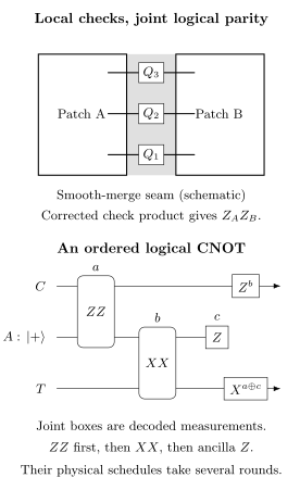
Top: local checks span an interface, and their corrected product yields a joint logical parity. The blocks are schematic, not a microscopic extraction circuit. Bottom: the ordered logical measurements implement CNOT after corrections $Z_C^b$ and $X_T^{a\oplus c}$. Each joint-measurement box expands into a protected schedule over several syndrome rounds.

Deriving the correction bits

Write $P=Z_CZ_A$ and $Q=X_AX_T$. The branch operator from the two input data qubits to the two output data qubits is

$$K_{abc}={}_A\langle c|\Pi_b^{(Q)} \Pi_a^{(P)}|+\rangle_A.$$

Define $\alpha=(-1)^{a+c}$ and $\beta=(-1)^b$. Evaluating the ancilla matrix elements gives

$$4\sqrt2 K_{abc}=I+\alpha Z_C+\beta X_T -\alpha\beta Z_CX_T.$$

For comparison,

$$\mathrm{CNOT}=\frac{I+Z_C+X_T-Z_CX_T}{2}.$$

Consequently, up to a branch-dependent global phase,

$$K_{abc}=\frac{1}{2\sqrt2} Z_C^bX_T^{a\oplus c}\,\mathrm{CNOT}.$$

Every branch has $K_{abc}^\dagger K_{abc}=I/8$, so all eight outcomes are equally likely for every data input. The record reveals no information about that input. Applying the two Pauli corrections gives a deterministic CNOT, including on states entangled with other systems.

Only two combinations of the three bits affect the correction:

$a\oplus c$	$b$	Correction
0	0	$I$
1	0	$X_T$
0	1	$Z_C$
1	1	$Z_CX_T$

These corrections can be applied physically or tracked in a Pauli frame. A different ancilla state, measurement ordering or sign convention requires rederiving the table. The logical derivation establishes the intended channel; it does not establish the reliability of its physical seam circuits.

Protecting the measurement in space and time

The interface must protect both the retained data and the reported parity. A circuit may preserve its quantum output but report the wrong parity, which then causes an incorrect correction in a later gate.

Repeated rounds provide temporal redundancy. For a persistent check with measurement bits $m_t$, changes $m_t\oplus m_{t-1}$ are detectors when the ideal check value is constant. An isolated readout error creates two changes in the bulk; a persistent data error can instead change the underlying check value.

A newly introduced check need not have a predetermined first result. Comparing it blindly with a fabricated previous zero creates a false detector. At a split, removed checks must connect correctly to single-qubit measurements and restored boundary checks. The transition record can also depend on faults that occurred before the merge.

Vuillot and collaborators (2019) describe deformation and surgery as gauge fixing. That viewpoint explains the changing constraints; Decoders explains inference over the resulting data-and-measurement fault histories.

Detection distance differs from correction radius

An operation’s circuit distance is often defined as the minimum number of elementary faults producing a nontrivial logical effect with no detector signature. In an appropriate binary fault model, it also constrains pairs of indistinguishable explanations. A minimum-weight decoder can guarantee correction of up to $\lfloor(D-1)/2\rfloor$ faults when their difference cannot contain an undetected logical combination of weight below $D$.

This is a stronger statement than inspecting one static patch, and a different statement from requiring $D$ faults before any decoded failure. For a simple repeated classical bit with three independent noisy copies, the undetected flip is the three-error word, yet two errors already cause majority decoding to fail. Exercise 4 computes this example explicitly.

Standard distance-$d$ surgery typically repeats the changed checks for order $d$ rounds. That temporal length is necessary in the usual repeated-readout construction, but does not prove operation distance $d$ by itself. A narrow route, a corner or an ancilla hook can provide a shorter spatial or mixed path. The exact preparation, gate order, measurement and final boundaries determine the distance.

Hooks arise when a check ancilla spreads one fault to several data qubits. Their orientation must be checked again when boundary checks change: a gate order safe in the bulk may be unsafe on a seam. Leakage and correlated faults require a model beyond independently sampled Pauli locations. A quoted memory threshold therefore cannot automatically be used as a surgery threshold.

Mixed Pauli products and routing

Surgery can measure products involving several patches, including mixed $X,Y,Z$ factors. An ancilla region reaches the relevant logical boundaries, and the combined checks reveal the desired product. Separated parts of the interface may be checked in parallel, so the number of participating patches does not by itself determine the number of serial rounds.

Mixed boundary types can introduce twists or domain-wall endpoints. Litinski and von Oppen (2018) construct surgery operations using these features. A $Y=iXZ$ factor needs a consistent phase and a joint physical construction; measuring $X$ and $Z$ separately is not a $Y$ measurement, since those observables do not commute. Twists can require different check weights and interaction schedules from a straight seam.

Patch rotation, additional ancilla regions and alternative measurement decompositions can trade spatial area against time. Litinski (2019) develops this description in terms of logical patch tiles. Such tiles simplify scheduling, but each represents many data and measurement qubits and repeated physical cycles.

For a fixed-size local operation, a patch area proportional to $d^2$ and duration proportional to $d$ syndrome cycles give qubit-cycle volume proportional to $d^3$. For a strip of physical length $L$ and width proportional to $d$,

$$A_{\rm strip}=O(Ld),\qquad V_{\rm strip}=O(Ld^2),$$

assuming parallel local checks for order $d$ cycles. If $L=Rd$ for separation $R$ measured in patch widths, the volume is $O(Rd^3)$. Parallel quantum checks can avoid serial traversal of the full length, but classical communication and decoding can still add distance-dependent latency. The cost is not independent of separation.

Larger routing regions can permit more simultaneous measurements; compact layouts can force serialization. Resource Estimation combines these choices with the workload. Magic State Distillation supplies resources whose delivery and consumption may occupy the same corridors.

Finally, a known Pauli frame can propagate through Clifford operations before it is fully resolved. The decision must arrive before an operation that actually depends on it, such as an adaptive non-Clifford basis choice. Not every surgery requires an immediate physical correction, and a favorable mean decoder speed does not guarantee every deadline. Current demonstrations and scaling questions are discussed in Fault-Tolerant Quantum Computing Frontier.

Exercises

1. Compare parity measurement with separate readout

Apply a $ZZ$ measurement to $|++\rangle$, condition on the even result, and compare with separate $Z$ measurements whose individual outcomes are subsequently discarded except for their parity.

Solution

The joint measurement gives the Bell state $(|00\rangle+|11\rangle)/\sqrt2$, with probability $1/2$. Separate readout conditioned on even parity gives

$$\rho_{\rm sep}=\tfrac12\bigl(|00\rangle\langle00| +|11\rangle\langle11|\bigr).$$

The Bell state has $\langle XX\rangle=1$; this mixture has $\langle XX\rangle=0$. Both have the same $ZZ$ eigenvalue, but different surviving coherence.

2. Track the dimension through merge and split

Using $V_m|j\rangle=|j,j\oplus m\rangle$, show that the two merge branches form a complete measurement and that splitting back gives the parity projectors.

Solution

Each $V_m$ has orthonormal columns and range equal to the parity-$m$ sector. Thus $V_mV_m^\dagger=\Pi_m$ and $V_m^\dagger V_m=I_2$. For $K_m=V_m^\dagger\Pi_m$,

$$\begin{aligned} \sum_m K_m^\dagger K_m&=\Pi_0+\Pi_1=I_4,\\ V_mK_m&=\Pi_m. \end{aligned}$$

The merge maps four input dimensions to two output dimensions in each branch. The classical outcome labels the selected sector. A subsequent split restores two physical logical qubits but cannot restore coherence between measured sectors.

3. Derive the CNOT branch operator

Evaluate the ancilla factors in $K_{abc}$ and recover its two Pauli byproducts.

Solution

For $c\in\{0,1\}$,

$$\begin{aligned} \langle c|+\rangle&=1/\sqrt2,\\ \langle c|Z|+\rangle&=(-1)^c/\sqrt2,\\ \langle c|X|+\rangle&=1/\sqrt2,\\ \langle c|XZ|+\rangle&=-(-1)^c/\sqrt2. \end{aligned}$$

The last minus sign comes from the order $XZ$ in the two sequential projectors. Substitution yields the displayed expansion with $\alpha=(-1)^{a+c}$ and $\beta=(-1)^b$. Comparing with CNOT gives correction $Z_C^bX_T^{a\oplus c}$. Its factors act on different qubits and commute. Multiplying by it makes every branch proportional to CNOT, with magnitude $1/(2\sqrt2)$.

4. Separate temporal distance from decoding failure

A constant classical bit is measured three times, with independent readout error probability $p<1/2$. Use adjacent differences as detectors and majority vote as the estimate. What is the smallest undetected nontrivial error, and what is the decoded failure probability?

Solution

The word $111$ flips all three readouts while leaving both differences unchanged, so the repetition distance is three. Majority vote nevertheless fails on any two-error word and on $111$:

$$\begin{aligned} p_{\rm fail}&=3p^2(1-p)+p^3\\ &=3p^2-2p^3. \end{aligned}$$

For example, observed $110$ is closer to constant one than constant zero, even though its detector record is nonzero. Distance three guarantees correction of one arbitrary error, not two. A full surgery record includes additional data faults and boundary information beyond this elementary model.

5. Test whether a split clones

Apply the smooth-split isometry to $|+\rangle$, find either reduced state, and compare its logical $X$ expectation with that of the input.

Solution

The output is $(|00\rangle+|11\rangle)/\sqrt2$. Either reduced state is $I/2$, so its individual $X$ expectation is zero. The input expectation was one, and it survives as $\langle X_1X_2\rangle=1$. The phase information resides in a correlation; neither daughter is a copy of the original pure state.

6. Count the cost of a long strip

A route has length $40d$, width $d$, and is checked for $d$ cycles. Ignore constant overheads. Compare its volume with one $d\times d$ patch stored for the same duration. What changes if its narrowest relevant logical path has length $d/2$?

Solution

The strip occupies $40d^2$ sites for $d$ cycles, giving $40d^3$ site-cycles. The stored patch costs $d^3$, so the ratio is forty. Parallel checks do not remove this area cost. If a nontrivial logical path has length $d/2$, the operation’s spatial protection is at most that value; extra rounds cannot repair the missing spatial width.

7. Propagate mistakes in the three outcome bits

Let the reported bits differ from the true CNOT measurement bits by $\delta a,\delta b,\delta c$. What residual Pauli remains after applying the reported correction?

Solution

Multiplying the true and reported byproducts cancels the known parts and leaves

$$Z_C^{\delta b}X_T^{\delta a\oplus\delta c}.$$

A wrong $b$ flips the control’s phase; a wrong $a$ or $c$ flips the target. If $a$ and $c$ are both wrong while $b$ is correct, their effects cancel. Thus the joint distribution of outcome errors matters, not only their individual rates.

8. Reverse the parity-measurement order

With ancilla $|+\rangle_A$, suppose $X_AX_T$ is measured before $Z_CZ_A$. Explain why this is not the same CNOT protocol.

Solution

Initially $X_A=+1$, so measuring $X_AX_T$ directly measures $X_T$. The outcome can depend on the unknown target state and destroys coherence between its $X$ sectors. A later correction cannot undo that measurement. By contrast, in the intended order the first parity measurement correlates A with C before the $XX$ step, and the complete three-bit record has input-independent probabilities. Algebraically the two parity observables anticommute, so swapping their projectors changes the branch maps.

References

• N. de Beaudrap and D. Horsman, “The ZX calculus is a language for surface code lattice surgery,” Quantum 4, 218 (2020), doi:10.22331/q-2020-01-09-218.
• D. Horsman, A. G. Fowler, S. Devitt, and R. Van Meter, “Surface code quantum computing by lattice surgery,” New Journal of Physics 14, 123011 (2012), doi:10.1088/1367-2630/14/12/123011, arXiv:1111.4022.
• D. Litinski, “A game of surface codes: large-scale quantum computing with lattice surgery,” Quantum 3, 128 (2019), doi:10.22331/q-2019-03-05-128, arXiv:1808.02892.
• D. Litinski and F. von Oppen, “Lattice surgery with a twist: simplifying Clifford gates of surface codes,” Quantum 2, 62 (2018), doi:10.22331/q-2018-05-04-62, arXiv:1709.02318.
• C. Vuillot, L. Lao, B. Criger, C. García Almudéver, K. Bertels, and B. M. Terhal, “Code deformation and lattice surgery are gauge fixing,” New Journal of Physics 21, 033028 (2019), doi:10.1088/1367-2630/ab0199, arXiv:1810.10037.