Decoding and Real-Time Control

A real-time decoder turns syndrome measurements into a recovery or a classical correction record before a later operation needs the answer. It must infer accurately, keep up with incoming data, and meet the relevant feedback deadlines. These are different requirements: even a decoder that is usually fast can make a computation wait after one difficult syndrome history.

Helpful background. Decoders explains the inference algorithms; mid-circuit measurement and feedforward explains adaptive circuit dependencies. This page analyzes their timing interface, rather than reproducing matching or belief-propagation algorithms.

Syndrome arrivals and decoder service

Suppose $B$ blocks each emit $m$ check records every $\tau$ seconds. The aggregate arrival rate is

$$\lambda=\frac{Bm}{\tau}.$$

This is a data rate, not necessarily a rate of independent decoding jobs: one job may combine many records and several rounds. For a single queue, define both arrival rate $\lambda_j$ and mean service rate $\mu_j$ in the same job units. Under the usual stationary stochastic queue assumptions, $\lambda_j<\mu_j$ provides the required capacity headroom. Equality can remain bounded in special deterministic schedules, but leaves no spare capacity to absorb variation. Neither a favorable mean rate nor a large raw-data bandwidth guarantees a deadline.

For an idealized M/M/1 queue of these jobs, with Poisson arrivals and independent exponential service times, the steady-state mean time from arrival to completion is

$$\mathbb E[T]=\frac{1}{\mu_j-\lambda_j}.$$

This elementary model illustrates sensitivity to utilization; actual syndrome streams are often periodic and decoder service times may be strongly nonexponential. At $90\%$ utilization the mean response is ten times the mean service time; at $99\%$ it is one hundred times. A capacity figure quoted without workload and queue behavior leaves a large uncertainty.

A deterministic example makes the distinction visible without a queueing approximation. Let one job arrive every unit of time, starting at $a_i=i-1$. Jobs are served in order by one engine. If $S_i$ is the service duration and $f_i$ its finishing time, then

$$f_i=\max(a_i,f_{i-1})+S_i,\qquad f_0=0.$$

For eight jobs with durations $(0.4,0.4,3,0.4,0.4,0.4,0.4,0.4)$, the average service time is only $0.725$. Yet the third job creates a queue: jobs three through six miss a deadline of one time unit after their respective arrivals. Even a later job needing only $0.4$ can be late because it first waits for the engine.

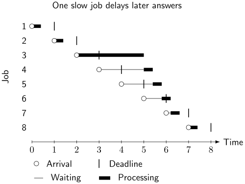
An illustrative single-engine schedule. A dot marks arrival, a gray line marks waiting, a black bar marks processing, and a vertical tick marks the deadline one unit after arrival. Average capacity is sufficient for this repeated pattern, but four jobs still miss their individual deadlines. Units are arbitrary; this is not a measured decoder trace.

Parallel engines can process spatial partitions or overlapping time windows. Fowler, Whiteside, and Hollenberg analyze local parallel classical processing for surface-code decoding. Boundary information must still be reconciled, and that reconciliation has both inference and communication costs. Splitting a decoding graph into independent pieces without accounting for boundary faults changes the error model.

A Pauli frame postpones some decisions

Many inferred Pauli corrections can be stored as classical frame updates rather than physically applied. Clifford operations transform such frames by known rules. This permits decoding to lag behind some quantum operations without immediately stopping the machine.

An adaptive non-Clifford operation, basis selection, or final interpretation may require a specific unresolved frame bit. The relevant deadline is the time from arrival of the necessary syndrome data to that dependency, not automatically one error-correction cycle. Conversely, finishing each typical cycle quickly does not establish safe behavior for the rare difficult histories that dominate failure.

Delfosse, Paz, Vaschillo, and Svore formulate decoder selection as an accuracy–speed tradeoff affecting spacetime cost. Their analysis motivates measuring performance for the intended logical depth and stopping policy, instead of ranking decoders solely by offline accuracy.

Put timeouts in the failure budget

Let $p_{\mathrm{wrong}}$ denote an incorrect decision returned on time and $p_{\mathrm{late}}$ the probability that a deadline is missed. Conservatively treating a missed deadline as a failed operation gives

$$p_{\mathrm{op}}\le p_{\mathrm{wrong}}+p_{\mathrm{late}}+p_{\mathrm{other}}.$$

The terms need not be independent for the union bound. If a late decision triggers a stall, one should instead model the extra memory channel during that stall. If it triggers an approximate answer, measure the resulting logical error. Counting timeouts as discarded data can make the advertised decoder error artificially small.

As a worked budget, consider $10^7$ sequential adaptive decisions with total timeout allocation $10^{-3}$. A union-bound allocation requires a per-decision timeout probability no larger than $10^{-10}$. Reporting only a 99.9th-percentile latency addresses a tail probability of $10^{-3}$, seven orders of magnitude larger. This does not show the controller fails; it shows the reported statistic cannot establish the required reliability.

Measuring a $10^{-10}$ tail directly is expensive. With zero observed misses in $N$ independent representative trials, the one-sided 95% binomial upper confidence limit is

$$p_{\mathrm{upper}}=1-0.05^{1/N}\approx\frac{3}{N}.$$

This is a statistical confidence statement, not a deterministic guarantee that the unknown probability is below the limit. Reaching $p_{\mathrm{upper}}\le10^{-10}$ with zero misses needs about $3.0\times10^{10}$ representative independent trials. A justified analytical bound can be more informative than direct sampling of such a rare tail. Independence and stationarity matter; replaying one easy trace repeatedly does not explore rare events.

Calibration changes the inference problem

Decoder weights encode a noise model. Drift, leakage, crosstalk, or changes in pulse schedules can invalidate it while the software continues to return plausible answers. A controller should track which calibration and circuit version generated each record and evaluate candidate weight updates on separate data.

Using training data to report the resulting logical performance biases the comparison. Updating aggressively on a few anomalous records can also amplify statistical fluctuations. Calibration loops treats feedback and drift; reporting standards explains how to report comparable measurements.

Causality, capacity, and the treatment of late or incorrect decisions are established requirements. Architecture-specific implementations remain an active engineering problem. The decoder research guide discusses selected implementations and open questions.

Exercises

A thousand blocks each produce 100 check records every $10\,\mu\mathrm{s}$. Each record occupies four bytes before transport overhead. Compute the raw input bandwidth.

Solution

The rate is $10^{10}$ records per second, giving $4\times10^{10}$ bytes per second, or $40$ GB/s in decimal units. Timestamps, framing, redundancy, and copying increase this budget. Decoder arithmetic throughput alone does not establish that the input path can sustain it.

A late result causes a $20\,\mu\mathrm{s}$ stall with probability $10^{-4}$. Conditional on a stall, assume a constant absorbing memory-failure hazard of $10\,\mathrm{s}^{-1}$. Estimate the additional failure per decision.

Solution

The conditional stall failure is $1-e^{-10(20\times10^{-6})}\approx2\times10^{-4}$. Multiplying by stall probability gives approximately $2\times10^{-8}$ per decision. This uses the stated hazard conditional on a stall. If difficult decoding histories also indicate noisier memories, an unconditional average memory rate cannot be substituted without checking that correlation. A Pauli flip rate with possible cancellation would require a different model.

In the plotted queue, when does the fourth job finish? Would dividing its own service duration by the average utilization predict its response time?

Solution

Job three finishes at $2+3=5$. Job four arrives at $3$, waits until $5$, and finishes at $5.4$. Its response time is therefore $2.4$, although its own service takes only $0.4$. A utilization average does not determine this individual waiting time; the preceding jobs and their arrival times matter.

Why does a 95% confidence limit based on zero misses become ten times smaller when the number of trials grows tenfold, rather than a hundredfold?

Solution

At a small candidate miss probability $p$, the zero-miss probability is $(1-p)^N\approx e^{-Np}$. Setting this equal to $0.05$ gives $p\approx-\log(0.05)/N$. The rare-event zero-count limit scales as $1/N$; it is not the usual fixed-variance standard-error calculation. The trials must still represent the future workload.

References

• N. Delfosse, A. Paz, A. Vaschillo, and K. M. Svore, “How to choose a decoder for a fault-tolerant quantum computer? The speed vs accuracy trade-off,” arXiv:2310.15313 (2023). Author preprint.
• A. G. Fowler, A. C. Whiteside, and L. C. L. Hollenberg, “Towards practical classical processing for the surface code,” Physical Review Letters 108, 180501 (2012). doi:10.1103/PhysRevLett.108.180501.

Further reading

Control, readout, and calibration follows the physical–classical loop; fault-tolerant gates identifies where adaptive dependencies enter.