Common Molecular Hamiltonians

A molecule can be described with all its electrons and nuclei, with nuclei moving on an electronic potential-energy surface, or with a small matrix of selected rotational and spin levels. Each description answers different questions. This reference compares their operators, assumptions, units, and angular-momentum conventions.

The key physical connection is that electronic binding determines a potential for nuclear motion. Vibration and rotation then emerge from that motion; they are not exactly independent because rotating a stretched molecule costs less energy than rotating a compact one at the same angular momentum.

Required background. Molecular Hamiltonian introduces the particle coordinates and Coulomb interactions. Helpful background. Atomic units explains the Hartree form used below. Brown and Carrington (2003) develop the spectroscopic reductions and spin conventions in detail.

Nonrelativistic Coulomb Hamiltonian

Let $N_e$ electrons have coordinates $\mathbf r_i$, and let $N_N$ nuclei have coordinates $\mathbf R_A$, charges $Z_Ae$, and masses $M_A$. In SI units, the spin-free point-particle Hamiltonian is

$$H_{\mathrm{lab}} ={} -\sum_i \frac{\hbar^2}{2m_e} \nabla_{\mathbf r_i}^2 -\sum_A \frac{\hbar^2}{2M_A} \nabla_{\mathbf R_A}^2 + \frac{e^2}{4\pi\epsilon_0} \left[ \sum_{i<j}\frac{1}{r_{ij}} +\sum_{A<B}\frac{Z_AZ_B}{R_{AB}} -\sum_{i,A}\frac{Z_A}{r_{iA}} \right].$$

Every coordinate is dynamical. In particular, the internuclear term is an operator on nuclear coordinates; it becomes a geometry-dependent scalar only in a clamped-nuclei electronic problem.

In Hartree atomic units,

$$H_{\mathrm{lab}} ={} -\frac12\sum_i\nabla_{\mathbf r_i}^2 -\sum_A \frac{1}{2M_A} \nabla_{\mathbf R_A}^2 + \sum_{i<j}\frac{1}{r_{ij}} +\sum_{A<B}\frac{Z_AZ_B}{R_{AB}} -\sum_{i,A}\frac{Z_A}{r_{iA}},$$

where every $M_A$ is expressed in electron-mass units. Atomic Units gives the unit dictionary and dimensional-restoration checks.

This spin-independent model omits relativistic, radiative, finite-nuclear-size, and applied-field effects. Spin still constrains the exchange symmetry of identical electrons and nuclei. An environment or quantized radiation field requires additional degrees of freedom.

Remove overall translation

For an isolated molecule with no external field,

$$H_{\mathrm{lab}} = \frac{\mathbf P_{\mathrm{cm}}^2}{2M_{\mathrm{tot}}} +H_{\mathrm{int}},$$

with

$$M_{\mathrm{tot}} = N_em_e+\sum_A M_A.$$

The internal Hamiltonian contains reduced masses and, depending on the coordinate choice, mass-polarization or other kinetic cross terms. Deleting a center-of-mass coordinate from the printed laboratory equation does not by itself derive $H_{\mathrm{int}}$.

This separation is exact for a translationally invariant isolated Hamiltonian. Homogeneous magnetic fields require more careful pseudomomentum and gauge treatment, especially for a charged molecule.

Born–Oppenheimer Electronic Hamiltonian

Two surface conventions

At fixed nuclear geometry $R$, define the electronic-only operator in atomic units by

$$H_{\mathrm{el}}(R) ={} -\frac12\sum_i\nabla_i^2 -\sum_{i,A}\frac{Z_A}{r_{iA}} + \sum_{i<j}\frac{1}{r_{ij}}.$$

Solve

$$H_{\mathrm{el}}(R) \phi_a(r;R) = \mathcal E_a(R) \phi_a(r;R).$$

The corresponding potential-energy surface is

$$U_a(R) = \mathcal E_a(R)+V_{NN}(R),$$

where

$$V_{NN}(R) = \sum_{A<B}\frac{Z_AZ_B}{R_{AB}}.$$

Another common convention includes $V_{NN}$ directly:

$$H_e(R) = H_{\mathrm{el}}(R)+V_{NN}(R), \qquad H_e(R)\phi_a = U_a(R)\phi_a.$$

Both conventions are correct. The error is to diagonalize the second operator and then add $V_{NN}$ again, or to diagonalize the first and forget it.

What is fixed and what remains quantum

During the electronic eigenproblem, $R$ is a parameter. The nuclei have not been declared classical forever; their quantum kinetic energy is restored in the nuclear equation. “Clamped nuclei” names an auxiliary problem, not a statement that a molecular eigenstate contains motionless nuclei.

At a fixed geometry, point-group labels and an electronic spin multiplicity may classify $\phi_a$. Over nuclear configuration space, labels can change, surfaces can approach one another, and a single adiabatic state may not provide a globally smooth basis.

Electronic Channels and Nuclear Motion

A complete geometry-dependent electronic basis gives

$$\Psi(r,R) = \sum_a \chi_a(R)\phi_a(r;R).$$

The expansion is exact for a complete electronic basis (including any required continuum); keeping only finitely many channels is a truncation. Acting with nuclear kinetic energy generates the coupled equations

$$\sum_b \left[ \left( T_N+U_a \right)\delta_{ab} +\tau_{ab} \right] \chi_b = E\chi_a,$$

where $\tau_{ab}$ contains diagonal and off-diagonal derivative couplings. In simple Cartesian notation,

$$\begin{aligned} \tau_{ab} = -\sum_A \frac{\hbar^2}{2M_A} \Big[ 2\mathbf d_{ab,A}\mathbin{\cdot}\nabla_A +D_{ab,A} \Big], \end{aligned}$$

with

$$\mathbf d_{ab,A} = \langle\phi_a\vert\nabla_A\phi_b\rangle_e, \qquad D_{ab,A} = \langle\phi_a\vert\nabla_A^2\phi_b\rangle_e.$$

The one-surface leading Hamiltonian is

$$H_{\mathrm{nuc}}^{(a)} = T_N+U_a(R).$$

It is obtained by neglecting couplings to other electronic channels and the geometry dependence of $\phi_a$ inside $T_N$. Adiabatic diagonal corrections, geometric vector potentials, and nonadiabatic couplings can be restored systematically, but their form depends on representation and gauge.

Nonadiabatic Coupling develops derivative couplings, adiabatic and diabatic representations, avoided crossings, and coupled nuclear dynamics.

One-surface validity

Compare the derivative coupling acting on the nuclear wavepacket with the electronic energy gap over the region that packet samples. The operators $\tau_{ab}$ contain derivatives, so their unrestricted operator norm is not a finite universal coupling constant. Faster nuclear motion can produce stronger channel mixing even for the same pair of surfaces.

A large gap at equilibrium alone is insufficient: a wavepacket may reach an avoided crossing or conical intersection elsewhere. Many individually small couplings can also accumulate; see the combined-coupling example. Diagonal geometric corrections and Berry phases may matter even when transitions to other surfaces are rare.

Nuclear Vibrational Hamiltonians

General internal-coordinate form

For internal coordinates $q^\mu$ with mass metric $G_{\mu\nu}(q)$, a coordinate-invariant kinetic operator has the schematic Laplace–Beltrami form

$$T_{\mathrm{nuc}} = -\frac{\hbar^2}{2} G^{-1/2} \partial_\mu \left[ G^{1/2} G^{\mu\nu} \partial_\nu \right],$$

where

$$G=\det G_{\mu\nu}.$$

The precise internal measure, removal of translation and rotation, body-fixed frame, and any ordering or pseudopotential terms must be derived for the selected coordinates. Replacing this operator by a Cartesian Laplacian in curvilinear coordinates is generally wrong.

Diatomic radial Hamiltonian

For a diatomic on an isolated $^1\Sigma$ electronic surface, neglecting nonadiabatic and diagonal geometric corrections, the reduced radial equation at rotational quantum number $N=J$ is

$$\Bigg[ - \frac{\hbar^2}{2\mu} \frac{d^2}{dR^2} +U_a(R) + \frac{\hbar^2N(N+1)} {2\mu R^2} \Bigg] u_{vN}(R) = E_{vN}u_{vN}(R),$$

where

$$\mu = \frac{M_AM_B}{M_A+M_B}.$$

Here the radial wavefunction is $u(R)/R$, so its normalization uses $\int_0^\infty|u(R)|^2\,dR=1$. States with nonzero electronic angular momentum need the corresponding rotational and electronic couplings; the displayed scalar equation is not their general Hamiltonian.

Setting $N=0$ gives the pure radial vibrational problem. Freezing $R=R_e$ gives the leading rigid rotor. The full equation already contains rotation–vibration coupling because the centrifugal term depends on the vibrational coordinate.

Vibrations of Diatomics develops anharmonic potentials, isotope scaling, Morse levels, and infrared transition moments.

Harmonic normal modes

Near a stable equilibrium, mass-weighted normal coordinates $Q_k$ reduce the quadratic vibrational Hamiltonian to

$$H_{\mathrm{vib}}^{(2)} = \frac12 \sum_{k=1}^{f} \left( P_k^2+\omega_k^2Q_k^2 \right),$$

with energies

$$E_{\{n_k\}} = \sum_{k=1}^{f} \hbar\omega_k \left( n_k+\frac12 \right).$$

For $N_N$ nuclei,

$$f = \begin{cases} 3N_N-5, & \text{linear molecule},\\ 3N_N-6, & \text{nonlinear molecule}. \end{cases}$$

The normal-mode basis is a local quadratic approximation. Anharmonicity, large-amplitude motion, resonances, tunneling, and vibronic coupling require a larger nuclear model. Normal Modes of Polyatomics develops the mass-weighted Hessian, symmetry classification, and activity criteria.

Rigid Rotor Hamiltonians

General top

For a nonlinear molecule at fixed reference geometry, let $\mathbf I$ be the inertia tensor about the center of mass. Neglecting shape motion gives

$$H_{\mathrm{rot}} = \frac12 \mathbf J_{\mathrm{rot}}^{\mathsf T} \mathbf I^{-1} \mathbf J_{\mathrm{rot}}.$$

In principal axes,

$$H_{\mathrm{rot}} = \frac{J_a^2}{2I_a} +\frac{J_b^2}{2I_b} +\frac{J_c^2}{2I_c}.$$

If $A$, $B$, and $C$ are frequency constants,

$$\frac{H_{\mathrm{rot}}}{h} = A\frac{J_a^2}{\hbar^2} +B\frac{J_b^2}{\hbar^2} +C\frac{J_c^2}{\hbar^2},$$

where

$$A=\frac{h}{8\pi^2I_a}, \qquad B=\frac{h}{8\pi^2I_b}, \qquad C=\frac{h}{8\pi^2I_c}.$$

Rotational constants in energy or wavenumber units differ by factors of $h$ or $hc$.

Rotor classes

Model	Moment relation	Spectral consequence
linear rotor	$I_a=0$, $I_b=I_c$	one scalar constant and a $J(J+1)$ ladder
spherical top	$I_a=I_b=I_c$	orientation has extra degeneracy
prolate symmetric top	$I_a<I_b=I_c$	exact body-axis projection $K$
oblate symmetric top	$I_a=I_b<I_c$	exact symmetry-axis projection $K$
asymmetric top	$I_a<I_b<I_c$	no exact $K$ and matrix diagonalization for each $J$

For a linear molecule the axial moment is zero, so do not insert its singular inertia tensor into the inverse above. There are only two physical orientational coordinates for an ideal linear rotor. For a closed-shell $^1\Sigma$ state,

$$\frac{H_{\mathrm{rot}}}{h} = B\frac{\mathbf J^2}{\hbar^2}, \qquad \frac{E_J}{h} = BJ(J+1).$$

For open-shell molecules, $J$ usually includes electronic spin while $N$ does not, so the spin-free rotational term is often written $B\mathbf N^2/\hbar^2$. Rotations of Molecules develops the conventions, rotor classes, centrifugal distortion, and spectroscopic inference in depth.

Vibration–Rotation Hamiltonians

The coupling is kinematic

In a semirigid polyatomic molecule, the inverse inertia tensor changes with internal coordinates. In a molecule-fixed frame, a useful schematic form is

$$H_{\mathrm{rv}} ={} H_{\mathrm{vib}} +\frac12 \sum_{\alpha,\beta} \mu_{\alpha\beta}(\mathbf q) \times \left( J_\alpha-\pi_\alpha \right) \left( J_\beta-\pi_\beta \right) +V_{\mathrm{ord}}(\mathbf q).$$

Here $\mu_{\alpha\beta}$ is a coordinate-dependent inverse inertia tensor, $\boldsymbol\pi$ is vibrational angular momentum, and $V_{\mathrm{ord}}$ denotes convention-dependent ordering or pseudopotential terms. An Eckart frame suppresses avoidable local coupling near a reference geometry; it does not remove physical Coriolis coupling.

Diatomic effective form

For a simple closed-shell diatomic, a common wavenumber expansion is

$$\frac{E_{vJ}}{hc} = \sum_{k,l} Y_{kl} \left( v+\frac12 \right)^k \left[ J(J+1) \right]^l.$$

The leading truncated form is

$$\frac{E_{vJ}}{hc} \approx G(v) +\widetilde B_vX -\widetilde D_vX^2, \qquad X=J(J+1),$$

with

$$\widetilde B_v = \widetilde B_e -\widetilde\alpha_e \left( v+\frac12 \right) +\cdots.$$

The mixed coefficients in the Dunham expansion and the $v$ dependence of $\widetilde B_v$ describe rotation–vibration coupling. This polynomial is a low-energy expansion: the truncated $\widetilde B_vX-\widetilde D_vX^2$ tends to $-\infty$ for arbitrarily large $J$ when $\widetilde D_v>0$, so it cannot predict the entire high-$J$ spectrum. Near dissociation, solve an appropriate nuclear-motion model.

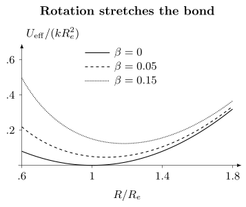
In the illustrative harmonic bond model, $U_{\mathrm{eff}}/(kR_e^2)=(x-1)^2/2+\beta/x^2$, where $x=R/R_e$ and $\beta=\hbar^2N(N+1)/(2\mu kR_e^4)$. Increasing angular momentum shifts the minimum to larger separation. The harmonic potential is a local model; these curves do not describe dissociation.

Effective Hamiltonians are representation dependent

For semirigid asymmetric tops, Watson $A$ and $S$ reductions remove redundant centrifugal-distortion parameters by different contact transformations. They predict the same spectrum to the retained order when used consistently, but their fitted constants need not agree term by term. Axis representations and sign conventions must also match.

Rovibrational Coupling develops Dunham organization, Coriolis effects, $P/Q/R$ branches, combination differences, branch heads, and fit diagnostics.

Angular-Momentum Dictionary

No molecular spin Hamiltonian is portable until its angular momenta are defined. A common diatomic convention is:

Symbol	Meaning
$\mathbf R$	end-over-end nuclear rotation
$\mathbf L$	total electronic orbital angular momentum
$\mathbf S$	total electronic spin
$\mathbf N$	total angular momentum excluding electronic spin and nuclear spin; often $\mathbf N=\mathbf J-\mathbf S$
$\mathbf J$	total angular momentum excluding nuclear spin
$\mathbf I_A$	spin of nucleus $A$
$\mathbf I$	coupled resultant of the nuclear spins
$\mathbf F$	total angular momentum including nuclear spin, usually $\mathbf F=\mathbf J+\mathbf I$

For a closed-shell $^1\Sigma$ state, $S=0$ and the simple rotational labels $N$ and $J$ coincide. In open-shell states, they do not. Some authors use $\mathbf N$ for bare rotation and others use it for all angular momentum except spin; the operator definitions, rather than the letter alone, are authoritative.

Fine and Spin–Rotation Terms

Electronic spin couplings

Within a selected electronic manifold, common effective fine-structure operators include

$$H_{\mathrm{fine}} ={} A_{\mathrm{so}} \frac{L_zS_z}{\hbar^2} + \frac{ \mathbf S \mathbin{\boldsymbol\cdot} \mathbf D \mathbin{\boldsymbol\cdot} \mathbf S }{\hbar^2} + \frac{ \mathbf N \mathbin{\boldsymbol\cdot} \boldsymbol\gamma \mathbin{\boldsymbol\cdot} \mathbf S }{\hbar^2} +\cdots.$$

The terms represent, respectively:

• effective spin–orbit coupling in an axial basis;
• electron spin–spin or zero-field splitting;
• electronic spin–rotation coupling.

Under this displayed normalization, $A_{\mathrm{so}}$ and the components of $\mathbf D$ and $\boldsymbol\gamma$ carry energy units. If the constants are quoted in hertz, divide the entire Hamiltonian by $h$.

For an idealized $^3\Sigma$ diatomic with constants in frequency units, a frequently used leading model is

$$\frac{H_{\mathrm{eff}}}{h} ={} B\frac{\mathbf N^2}{\hbar^2} +\frac{2\lambda}{3} \frac{ 3S_z^2-\mathbf S^2 }{\hbar^2} + \gamma \frac{ \mathbf N\mathbin{\boldsymbol\cdot}\mathbf S }{\hbar^2}.$$

This compact form is state-specific. Centrifugal corrections, vibrational dependence, spin–orbit mixing with other electronic states, and hyperfine terms may be required at higher resolution.

Electronic versus nuclear spin–rotation

The electronic term is

$$H_{\mathrm{esr}} = \frac{ \mathbf N \mathbin{\boldsymbol\cdot} \boldsymbol\gamma \mathbin{\boldsymbol\cdot} \mathbf S }{\hbar^2}.$$

The nuclear spin–rotation term is instead

$$H_{\mathrm{nsr}} = \sum_A \frac{ \mathbf I_A \mathbin{\boldsymbol\cdot} \mathbf C_A \mathbin{\boldsymbol\cdot} \mathbf N }{\hbar^2}.$$

The first can exist only when $S\ne0$. The second can split a closed-shell $^1\Sigma$ rotational level when $I_A\ne0$ and $N>0$. Its isotropic first-order contribution vanishes in an $N=0$ level. Both are often called “spin–rotation,” so the spin operator must always be printed.

Molecular Hyperfine Hamiltonian

At leading electromagnetic multipole order, a schematic molecular hyperfine Hamiltonian is

$$\begin{aligned} H_{\mathrm{hfs}} ={}& \sum_A b_{F,A} \frac{ \mathbf I_A\mathbin{\boldsymbol\cdot}\mathbf S }{\hbar^2} \\ &+ \sum_A \frac{ \mathbf I_A \mathbin{\boldsymbol\cdot} \mathbf T_A \mathbin{\boldsymbol\cdot} \mathbf S }{\hbar^2} \\ &+ \sum_A T^{(2)}(Q_A) \mathbin{\boldsymbol\cdot} T^{(2)}(\nabla\mathbf E_A) \\ &+ \sum_A \frac{ \mathbf I_A \mathbin{\boldsymbol\cdot} \mathbf C_A \mathbin{\boldsymbol\cdot} \mathbf N }{\hbar^2} \\ &+ \sum_{A<B} \frac{ \mathbf I_A \mathbin{\boldsymbol\cdot} \mathbf D_{AB} \mathbin{\boldsymbol\cdot} \mathbf I_B }{\hbar^2} +\cdots. \end{aligned}$$

The displayed normalization is schematic: authors distribute factors of $h$, $\hbar$, nuclear moments, and tensor normalizations differently.

Interaction	Physical source	Required angular momentum
Fermi contact	electron spin density at a nucleus	$S\ne0$, $I_A\ne0$
electron–nuclear dipolar	anisotropic magnetic dipole coupling	$S\ne0$, $I_A\ne0$
nuclear electric quadrupole	nuclear quadrupole with molecular electric-field gradient	$I_A\ge1$
nuclear spin–rotation	nuclear magnetic moment with field generated by molecular rotation	$I_A\ne0$
nuclear spin–spin	magnetic coupling between nuclei	at least two nonzero nuclear spins

Nuclear spin–orbit and higher nuclear multipoles may also enter specialized models. The nuclear electric-quadrupole term is a rank-2 tensor interaction; the familiar scalar constant $eQq$ is obtained only after choosing molecular axes and a tensor convention.

State dependence and vibrational averaging

Hyperfine constants are generally functions of geometry. A constant reported for vibrational level $v$ represents a matrix element such as

$$b_{F,v} = \langle \chi_v \vert b_F(R) \vert \chi_v \rangle,$$

possibly after further electronic-state projection and effective transformations. It is not automatically the value at $R_e$.

The NIST $^1\Sigma$ diatomic compilation uses separate constants for nuclear quadrupole, nuclear spin–rotation, and nuclear spin–spin effects. The NIST $^3\Sigma$ compilation also displays the electron spin–spin and electron spin–rotation terms. These provide explicit operator conventions for comparing reported constants.

External-Field Additions

For a neutral molecule in static, spatially slowly varying fields, common leading terms within a selected electronic manifold are

$$H_{\mathrm{field}} ={} -\boldsymbol\mu \mathbin{\boldsymbol\cdot} \mathbf E -\frac12 \mathbf E \mathbin{\boldsymbol\cdot} \boldsymbol\alpha \mathbin{\boldsymbol\cdot} \mathbf E - \boldsymbol\mu_{\mathrm{mag}} \mathbin{\boldsymbol\cdot} \mathbf B +\cdots.$$

Here $\boldsymbol\alpha$ represents the response of states omitted from the model, usually remote electronic states. Do not include the same rotational or electronic response both in $\boldsymbol\alpha$ and through explicit dipole-coupled states. For a far-off-resonant monochromatic field with real peak amplitude $\mathbf E_0$, the cycle-averaged scalar shift is $-\alpha(\omega)E_0^2/4$, not the static $-\alpha E^2/2$ with the peak amplitude inserted unchanged.

The molecular dipole and polarizability are body-fixed tensors, while the applied fields are usually specified in the laboratory frame. Direction cosines or spherical tensors connect the two. A static electric field mixes opposite-parity rotor states; a magnetic field can decouple angular momenta that were useful at zero field.

For charged molecules, center-of-mass and internal electric or magnetic couplings require an explicit gauge and coordinate derivation. A neutral internal dipole is origin independent, while an ionic dipole is not unless the center-of-mass convention is fixed.

Symmetries and Good Labels

Model	Exact or robust labels	Labels that are conditional
isolated spin-free Coulomb molecule	total spatial angular momentum, parity, permutation symmetry	equilibrium point group and body-fixed geometry
fixed-geometry electronic problem	geometry point-group irrep, electron exchange symmetry	energy ordering as a state label
one scalar surface for a nondegenerate electronic state	total rotational symmetry and permutation–inversion symmetry, when preserved by the reduction	separate vibrational and rotational quanta; electronic geometric phases can require a richer model
harmonic normal modes	mode occupation within the quadratic model	local-mode character outside the harmonic region
linear or symmetric rigid rotor	$J$ and an allowed projection label	vibrational state independence of constants
asymmetric rotor	$J$, $M$, parity, exact molecular symmetry	$K_a$ and $K_c$ as exact projections
field-free spin-resolved model	$F$ and parity when all retained terms are rotational scalars	intermediate couplings such as $N$, $J$, or the resultant $I$
molecule in a dc field	projection on the field axis under axial symmetry	zero-field parity and coupled angular momenta

The individual nuclear spins $I_A$ are fixed properties of the isotopes when nuclear internal excitation is excluded; the resultant of several nuclear spins need not be conserved. Exact labels depend on the Hamiltonian. When an interaction is added, states with the same exact symmetry may mix and their approximate labels may exchange character.

Molecular Symmetry develops point groups, irreducible representations, permutation–inversion issues, and spectroscopic selection rules.

Perturb or Diagonalize

After rephasing the basis to make the coupling real and positive, write

$$H=\begin{pmatrix}0&|V|\\ |V|&\Delta\end{pmatrix},\qquad\Delta>0.$$

Its lower eigenstate is $\cos\theta|1\rangle-\sin\theta|2\rangle$, with

$$\tan2\theta=\frac{2|V|}{\Delta},\qquad0\le\theta<\frac\pi4.$$

Nondegenerate perturbation theory requires $|V|/\Delta\ll1$. A small interaction measured in megahertz can therefore cause large mixing near a degeneracy. First separate exact symmetry sectors, then keep the coupled near-degenerate states in the same matrix. When eliminating states, transform the observables too. Refitted constants may be needed if the old effective constants already included the eliminated interaction.

Unit Conventions

The same operator may be reported in four common forms.

Printed object	Eigenvalue unit	Evolution factor
$H$	joule, electronvolt, or Hartree	$\exp(-iEt/\hbar)$
$H/h$	hertz	$\exp(-i2\pi\nu t)$
$H/\hbar$	radians per second	$\exp(-i\omega t)$
$H/(hc)$	inverse length, usually $\mathrm{cm}^{-1}$	convert through $E=hc\widetilde\nu$

Thus

$$E = h\nu = \hbar\omega = hc\widetilde\nu, \qquad \omega=2\pi\nu.$$

For a moment of inertia $I$,

$$B_E = \frac{\hbar^2}{2I}, \qquad B_\nu = \frac{h}{8\pi^2I}, \qquad \widetilde B = \frac{h}{8\pi^2cI}.$$

Never insert a hertz-valued $B_\nu$ into an energy Hamiltonian without multiplying by $h$. Constants and Conversions gives the corresponding $\mathrm{Hz}$, $\mathrm{cm}^{-1}$, electronvolt, kelvin, and angular-frequency conversions.

Common pitfalls

Using a fitted constant outside its range. A rotational or hyperfine constant can be vibrationally averaged and can absorb other state couplings. It need not equal its value at equilibrium. Check the isotope, vibrational state, and fitted quantum-number range before extrapolating.

Reading an equilibrium point group as the whole molecular symmetry. Point-group labels classify the fixed-geometry electronic problem. A freely rotating or tunneling molecule also needs rotational and permutation–inversion symmetry; see Molecular symmetry.

Comparing incompatible constants. The operators, units, axis convention, and effective-Hamiltonian reduction must match. Two equivalent reductions can give the same spectrum with different numerical parameters.

Worked Diagnostics

Closed-shell polar diatomic

For a $^1\Sigma$ molecule with one quadrupolar nucleus:

• $S=0$, so electronic spin–orbit, electron spin–spin, electronic spin–rotation, Fermi-contact, and electron–nuclear dipolar terms vanish in the isolated-state model;
• rotation, nuclear electric quadrupole, and nuclear spin–rotation remain;
• a static electric field can mix opposite-parity rotational states through $-\boldsymbol\mu\mathbin{\boldsymbol\cdot}\mathbf E$;
• at zero field, coupling $\mathbf F=\mathbf J+\mathbf I$ is useful when the retained hyperfine Hamiltonian is rotationally invariant.

“Closed shell” therefore does not mean “no hyperfine structure.”

Exercises

Count the nuclear repulsion once

A program reports the eigenvalue of

$$H_e = T_e+V_{eN}+V_{ee}+V_{NN}$$

as $-75.0\,E_h$ at one geometry. A script then adds $V_{NN}=9.0\,E_h$ to obtain the potential. Identify the error and the reported value that should enter the leading nuclear Hamiltonian.

Solution

Because $V_{NN}$ is already inside $H_e$, its eigenvalue is already the surface value in this convention. Adding $9.0\,E_h$ again double counts internuclear repulsion. The leading nuclear Hamiltonian should use

$$U(R)=-75.0\,E_h.$$

If the electronic operator had excluded $V_{NN}$, then adding it once would have been required.

Expose rotation–vibration coupling

Expand the diatomic centrifugal factor $1/R^2$ through second order in $q=R-R_e$. Identify the terms that couple vibration to rotation.

Solution

Using $(1+x)^{-2}=1-2x+3x^2+\cdots$,

$$\frac{1}{R^2} = \frac{1}{R_e^2} \left[ 1 -2\frac{q}{R_e} +3\frac{q^2}{R_e^2} +\cdots \right].$$

Therefore,

$$\frac{\hbar^2J(J+1)}{2\mu R^2} = B_EJ(J+1) +\left[ -2B_E\frac{q}{R_e} +3B_E\frac{q^2}{R_e^2} +\cdots \right] J(J+1).$$

Here $B_E=\hbar^2/(2\mu R_e^2)$ is an energy, unlike the frequency-valued $B$ used in the rotor section. The constant term is the equilibrium rigid rotor. The terms proportional to $qJ(J+1)$, $q^2J(J+1)$, and higher powers are explicit rotation–vibration couplings.

Leading isotope scaling

Two isotopologues have reduced masses $\mu'$ and $\mu''=4\mu'$. Assuming the same Born–Oppenheimer surface and equilibrium geometry, find $\omega_e''/\omega_e'$ and $B_e''/B_e'$.

Solution

The harmonic frequency scales as $\mu^{-1/2}$, while the rotational constant scales as $\mu^{-1}$:

$$\frac{\omega_e''}{\omega_e'} = \left( \frac{\mu'}{\mu''} \right)^{1/2} = \frac12,$$

and

$$\frac{B_e''}{B_e'} = \frac{\mu'}{\mu''} = \frac14.$$

These are leading mass laws, not exact high-precision isotope identities.

Nuclear spin–rotation in a closed shell

In a $^1\Sigma$ diatomic with one spin-$1$ nucleus, let $H_{\mathrm{nsr}}=C\mathbf I\cdot\mathbf N/\hbar^2$, where $C$ is an energy. Find the shifts for $N=1$ and compare with $N=0$.

Solution

Electronic spin–rotation vanishes because $S=0$, but nuclear spin remains. For $N=I=1$, the values $F=0,1,2$ have energies

$$E_F=\frac C2[F(F+1)-I(I+1)-N(N+1)] =-2C,-C,C.$$

The respective degeneracies $1,3,5$ give zero weighted centroid. For $N=0$, only $F=I=1$ occurs and this first-order interaction vanishes. Electric-quadrupole and other hyperfine terms are separate contributions.

Perturb or diagonalize

Two same-symmetry rovibronic levels are separated by $\Delta/h=4\,\mathrm{MHz}$ and coupled by $V/h=3\,\mathrm{MHz}$. Is nondegenerate perturbation theory reliable?

Solution

The mixing criterion is

$$\frac{2|V|}{|\Delta|} = \frac{6}{4} = 1.5.$$

This is not small. The mixing angle satisfies

$$\tan2\theta=1.5,\qquad\theta\simeq28.15^\circ.$$

The eigenvalue separation is $\sqrt{\Delta^2+4|V|^2}/h\simeq7.21\,\mathrm{MHz}$, and the lower state has $\sin^2\theta\simeq0.223$ weight in the upper unperturbed level. Both levels belong in the retained model space and the $2\times2$ block should be diagonalized. Calling the coupling “only a few megahertz” is irrelevant without comparing it with the allowed-state gap.

References

• Brown, J. M., and A. Carrington. Rotational Spectroscopy of Diatomic Molecules. Cambridge University Press, 2003. DOI.
• Dunham, J. L. “The Energy Levels of a Rotating Vibrator.” Physical Review 41, 721–731 (1932). DOI.
• National Institute of Standards and Technology. Diatomic Spectral Database: singlet-Sigma ground states and triplet-Sigma ground states. Operator conventions and evaluated constants; accessed 14 October 2026.