Line Shape Reference

A linewidth describes the spread of a spectral feature. To interpret it, identify the spectral axis, the definition of width, and the measured quantity. For example, an excited-state lifetime of $30$ ns gives a natural full width of $5.31$ MHz when the lower state is stable and pure dephasing is absent. The decay rate itself is $3.33\times10^7\ \mathrm{s^{-1}}$.

This reference collects isolated-line formulas and their assumptions. For the reasoning behind them, see Line Shapes and Broadening.

Helpful background. Line Shapes and Broadening explains how coherence decay and a distribution of resonance frequencies produce different profiles.

Spectral coordinates and widths

Unless a section says otherwise, use angular frequency

$$x = \delta\omega = \omega-\omega_0$$

and the following symbols:

Symbol	Meaning	Units on an angular-frequency axis
$\gamma_{\mathrm L}$	Lorentzian HWHM	$\mathrm{rad\,s^{-1}}$
$w_{\mathrm L}=2\gamma_{\mathrm L}$	Lorentzian FWHM	$\mathrm{rad\,s^{-1}}$
$\sigma_{\mathrm G}$	Gaussian standard deviation	$\mathrm{rad\,s^{-1}}$
$w_{\mathrm G}$	Gaussian FWHM	$\mathrm{rad\,s^{-1}}$
$\Gamma_1$	population-decay rate	$\mathrm{s^{-1}}$
$\Gamma_2$	coherence-decay rate	$\mathrm{s^{-1}}$
$T_1=1/\Gamma_1$	population lifetime	$\mathrm s$
$T_2=1/\Gamma_2$	coherence time	$\mathrm s$

Radians are dimensionless in SI, but retaining rad in a label makes the $2\pi$ convention visible.

Coordinate conversions

Angular frequency $\omega$, ordinary frequency $\nu$, photon energy $E$, and spectroscopic wavenumber $\widetilde\nu$ obey

$$\omega=2\pi\nu, \qquad E=h\nu=\hbar\omega, \qquad \nu=c\widetilde\nu.$$

These coordinate changes are linear, so corresponding widths satisfy exactly

$$\Delta\omega = 2\pi\Delta\nu,$$ $$\Delta E = \hbar\Delta\omega = h\Delta\nu,$$ $$\Delta\widetilde\nu = \frac{\Delta\nu}{c}.$$

Do not use $\widetilde\nu$ for ordinary frequency merely because both are pronounced “nu.” Spectroscopic wavenumber is commonly reported in $\mathrm{cm^{-1}}$.

Width vocabulary

Name	Definition	Symmetric-profile relation
peak center	location of maximum	equals the location parameter only for the stated symmetric model
HWHM	positive offset at half maximum	$x_{1/2}$
FWHM	distance between the two half-maximum points	$2x_{1/2}$
standard deviation	square root of second central moment	finite for a Gaussian; undefined for an ideal Lorentzian
$1/e$ half width	offset where the profile falls to $1/e$ of peak	profile dependent
equivalent width	integrated absorption relative to a continuum	not a line-profile FWHM

The symbol $\Gamma$ has no universal width meaning. Always replace it with a named HWHM, FWHM, decay rate, or energy width when comparing sources.

Normalized Profiles

Let $g_x(x)$ be a line profile normalized on coordinate $x$:

$$\int_{-\infty}^{\infty} g_x(x)\,dx = 1.$$

Its units are the reciprocal units of $x$. A spectral power density can be written $P_x(x)=P_{\mathrm{tot}}g_x(x)$, where $P_{\mathrm{tot}}$ is the integrated power. The area stays fixed while the profile redistributes it. Peak height and width are therefore not independent at fixed area.

Changing the spectral coordinate

For a monotonic change $y=y(x)$, a normalized density transforms as

$$g_y(y)=g_x\!\bigl(x(y)\bigr)\left|\frac{dx}{dy}\right|.$$

For positive vacuum frequencies and wavelengths,

$$\nu=\frac{c}{\lambda},\qquad P_\lambda(\lambda)=P_\nu(c/\lambda)\frac{c}{\lambda^2}.$$

The Jacobian ensures that integrating either density over the same spectral interval gives the same power. The ideal profiles below extend detuning to the whole real line; for an optical line this is a local approximation near a positive carrier. Do not apply a wavelength transformation to their unphysical negative-frequency tails.

A monochromatic attenuation coefficient is a different object. In $I_{\rm out}(\nu)=I_{\rm in}(\nu)e^{-\alpha(\nu)\ell}$, the coefficient $\alpha$ is the attenuation per length at a specified frequency. Relabeling the same light by wavelength gives

$$\alpha_\lambda(\lambda)=\alpha_\nu(c/\lambda),$$

with no Jacobian. Both incident and transmitted spectral power densities acquire the same Jacobian, which cancels in their ratio. An integrated absorption strength such as $\int\alpha_\nu\,d\nu$ consequently depends on the chosen coordinate. In a formula $\alpha_\nu=S_\nu g_\nu$, define $S_\nu$ using that same coordinate.

A frequency-symmetric profile generally becomes asymmetric in wavelength. The useful width relation

$$\frac{|\Delta\lambda|}{\lambda_0}\simeq \frac{|\Delta\nu|}{\nu_0}$$

is only a first-order narrow-line approximation.

Profile Comparison

Property	Lorentzian	Gaussian	Voigt
parameters	center and HWHM $\gamma_{\mathrm L}$	center and standard deviation $\sigma_{\mathrm G}$	center, $\gamma_{\mathrm L}$, and $\sigma_{\mathrm G}$
common origin	exponential coherence, isolated damped pole, impact-limit phase interruption	normal distribution of static shifts, thermal one-axis velocities, Gaussian instrument response	independent Gaussian and Lorentzian stages
wings	algebraic, proportional to $x^{-2}$	exponential in $-x^2$	Lorentzian asymptote if $\gamma_{\mathrm L}>0$
variance	does not exist on an infinite domain	$\sigma_{\mathrm G}^2$	does not exist if $\gamma_{\mathrm L}>0$
convolution with the same family	HWHMs add	variances add	HWHMs add and Gaussian variances add
one-width description	HWHM or FWHM is sufficient after normalization	standard deviation or FWHM is sufficient after normalization	requires both component widths

Similar-looking cores do not imply similar wings. This matters for weak neighboring lines, optical-depth retrievals, and truncated fit windows.

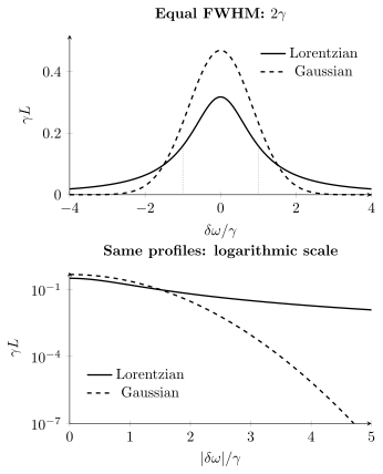
Both curves have unit area and the same full width $2\gamma$. Their peak heights differ because the Lorentzian puts more area into its wings. The lower panel shows how rapidly the Gaussian becomes small away from line center. The plotted ordinate is $\gamma$ times each normalized profile.

Lorentzian

The area-normalized Lorentzian is

$$L(x;\gamma_{\mathrm L}) = \frac{1}{\pi} \frac{\gamma_{\mathrm L}} {x^2+\gamma_{\mathrm L}^2}.$$

Its lookup properties are:

$$L(0) = \frac{1}{\pi\gamma_{\mathrm L}},$$ $$\text{HWHM} = \gamma_{\mathrm L}, \qquad \text{FWHM} = w_{\mathrm L} = 2\gamma_{\mathrm L},$$ $$L(x) \sim \frac{\gamma_{\mathrm L}} {\pi x^2} \qquad (|x|\gg\gamma_{\mathrm L}).$$

A Lorentzian does not have a finite ordinary variance:

$$\int_{-\infty}^{\infty} x^2L(x)\,dx \quad\text{diverges}.$$

Consequently, a reported “Lorentzian standard deviation” either refers to a finite window, a different distribution, or an undocumented convention.

Coherence time and spectral width

An exponentially decaying coherence

$$C(t) \propto e^{-\Gamma_2|t|} e^{-i\omega_0t}$$

produces a Lorentzian frequency dependence with

$$\gamma_{\mathrm L,\omega} = \Gamma_2,$$

and hence

$$w_{\mathrm L,\omega} = 2\Gamma_2 = \frac{2}{T_2}.$$

On an ordinary-frequency axis,

$$\gamma_{\mathrm L,\nu} = \frac{\Gamma_2}{2\pi},$$ $$w_{\mathrm L,\nu} = \frac{\Gamma_2}{\pi} = \frac{1}{\pi T_2}.$$

These relations assume exponential coherence over the times relevant to the measurement.

Gaussian

The area-normalized Gaussian is

$$G(x;\sigma_{\mathrm G}) = \frac{1} {\sigma_{\mathrm G}\sqrt{2\pi}} \exp\!\left( -\frac{x^2} {2\sigma_{\mathrm G}^2} \right).$$

Its lookup properties are:

$$G(0) = \frac{1} {\sigma_{\mathrm G}\sqrt{2\pi}},$$ $$\text{HWHM} = \sqrt{2\ln2}\, \sigma_{\mathrm G},$$ $$w_{\mathrm G} = 2\sqrt{2\ln2}\, \sigma_{\mathrm G}.$$

Numerically,

$$w_{\mathrm G} \simeq 2.35482\,\sigma_{\mathrm G}.$$

The $1/e$ half width is

$$x_{1/e} = \sqrt2\,\sigma_{\mathrm G}.$$

Do not confuse this with the half width at half maximum.

Combining Gaussian stages

For independent Gaussian shifts,

$$\sigma_{\mathrm{tot}}^2 = \sum_i\sigma_i^2.$$

Because every Gaussian FWHM contains the same multiplicative factor,

$$w_{\mathrm{G,tot}}^2 = \sum_i w_{\mathrm{G},i}^2.$$

This quadrature rule applies to Gaussian convolution parameters. It is not a generic rule for all quoted uncertainties or all spectral widths.

Voigt

The Voigt profile is the convolution of a Gaussian and a Lorentzian (NIST DLMF, §7.19):

$$V(x;\sigma_{\mathrm G},\gamma_{\mathrm L}) = \int_{-\infty}^{\infty} G(x';\sigma_{\mathrm G}) \times L(x-x';\gamma_{\mathrm L}) \,dx'.$$

It is area normalized if both components are normalized.

Faddeeva representation

Define

$$w(z) = e^{-z^2} \operatorname{erfc}(-iz),$$

and

$$z = \frac{x+i\gamma_{\mathrm L}} {\sigma_{\mathrm G}\sqrt2}.$$

Then

$$V(x;\sigma_{\mathrm G},\gamma_{\mathrm L}) = \frac{ \operatorname{Re}w(z) } {\sigma_{\mathrm G}\sqrt{2\pi}}.$$

Use a tested complex-error-function implementation. Direct numerical quadrature or naive evaluation of $e^{-z^2}\operatorname{erfc}(-iz)$ can lose accuracy in parts of the complex plane.

Limits

The Voigt profile has the expected limits:

$$\lim_{\gamma_{\mathrm L}\to0} V(x;\sigma_{\mathrm G},\gamma_{\mathrm L}) = G(x;\sigma_{\mathrm G}),$$ $$\lim_{\sigma_{\mathrm G}\to0} V(x;\sigma_{\mathrm G},\gamma_{\mathrm L}) = L(x;\gamma_{\mathrm L}).$$

Any nonzero $\gamma_{\mathrm L}$ controls the far-wing asymptote, even when the core looks nearly Gaussian.

Approximate Voigt FWHM

Let

$$w_{\mathrm L}=2\gamma_{\mathrm L}, \qquad w_{\mathrm G} = 2\sqrt{2\ln2}\,\sigma_{\mathrm G}.$$

The approximation discussed by Olivero and Longbothum (1977) is

$$w_{\mathrm V} \simeq 0.5346\,w_{\mathrm L} + \sqrt{ 0.2166\,w_{\mathrm L}^2 + w_{\mathrm G}^2 }.$$

This estimates the resulting FWHM. It does not convert a fitted single $w_{\mathrm V}$ into unique Lorentzian and Gaussian components.

Voigt is not pseudo-Voigt

A pseudo-Voigt profile is a weighted sum,

$$P(x) = \eta L(x) + (1-\eta)G(x),$$

with widths arranged according to a chosen approximation. A Voigt profile is a convolution. A pseudo-Voigt can be computationally convenient, but its mixing fraction $\eta$ is not a physical Lorentzian fraction unless a particular model establishes that interpretation.

Width-Combination Rules

Independent stages	Correct combination	Resulting family
Lorentzian + Lorentzian	add HWHMs: $\gamma_{\mathrm{tot}}=\gamma_1+\gamma_2$	Lorentzian
Gaussian + Gaussian	add variances: $\sigma_{\mathrm{tot}}^2=\sigma_1^2+\sigma_2^2$	Gaussian
Lorentzian + Gaussian	convolve	Voigt
Voigt + Voigt	add Lorentzian HWHMs and Gaussian variances separately	Voigt
unresolved discrete components	sum shifted component profiles with weights	generally not one standard profile
saturation plus Doppler distribution	average the intensity-dependent response over velocities	not automatically a fixed Voigt
line mixing or interference	use coupled response amplitudes or a relaxation matrix	can be asymmetric or dispersive

Blindly adding all FWHMs linearly is wrong. Blindly adding all FWHMs in quadrature is also wrong. First classify the profile family and statistical relationship.

Natural and Lifetime Width

For a transition between upper and lower levels with population-loss rates $\Gamma_u$ and $\Gamma_l$, and with additional Markovian pure dephasing $\gamma_\phi$, independent population-loss channels give

$$\Gamma_2 = \frac{\Gamma_u+\Gamma_l}{2} + \gamma_\phi.$$

The Lorentzian angular-frequency widths are

$$\gamma_{\mathrm L,\omega} = \Gamma_2,$$ $$w_{\mathrm L,\omega} = 2\Gamma_2 = \Gamma_u+\Gamma_l+2\gamma_\phi.$$

On an ordinary-frequency axis,

$$w_{\mathrm L,\nu} = \frac{ \Gamma_u+\Gamma_l+2\gamma_\phi } {2\pi}.$$

This assumes an isolated optical coherence with no coupling to other coherences. Shared reservoirs, correlated noise, or nearly degenerate transitions can require a coupled master equation instead.

Simplest natural-width limit

If the lower state is stable, the upper state decays only radiatively, and there is no pure dephasing,

$$\Gamma_l=0, \qquad \gamma_\phi=0,$$ $$\Gamma_u = \sum_l A_{ul} = \frac{1}{\tau_u}.$$

Then

$$w_{\mathrm{nat},\omega} = \Gamma_u,$$ $$\Delta\nu_{\mathrm{nat}} = \frac{\Gamma_u}{2\pi} = \frac{1}{2\pi\tau_u},$$ $$\Delta E_{\mathrm{nat}} = \hbar\Gamma_u.$$

The relation “linewidth equals inverse lifetime” is correct here only for angular-frequency FWHM. The ordinary-frequency FWHM contains $2\pi$.

What counts as lifetime loss

The total upper-state loss can include

$$\Gamma_u^{\mathrm{tot}} = \Gamma_u^{\mathrm{rad}} + \Gamma_u^{\mathrm{nr}},$$

where nonradiative loss may include quenching, predissociation, autoionization, reaction, or escape from the selected state. Such loss can broaden the transition without contributing to the detected fluorescence branch.

“Natural linewidth” should identify the electromagnetic environment. Cavities and structured reservoirs can modify radiative decay, while strong coupling can replace one broadened peak with resolved normal modes.

Doppler Width

For a thermal gas in equilibrium, one velocity component is Gaussian with variance

$$\sigma_v^2 = \frac{k_{\mathrm B}T}{m}.$$

For a wavevector of magnitude

$$k_0 = \frac{\omega_0}{c},$$

a particle moving with velocity component $v_\parallel$ along the beam sees the rest-frame detuning

$$\Delta_{\rm atom}\simeq\omega_{\rm L}-k_0v_\parallel-\omega_0.$$

Its resonance therefore occurs at the laboratory frequency $\omega_{\rm L}\simeq\omega_0+k_0v_\parallel$. The sign distinguishes a shift of the laser frequency in the particle frame from a shift of the laboratory resonance.

The angular-frequency standard deviation is therefore

$$\sigma_{\mathrm D,\omega} = \frac{\omega_0}{c} \sqrt{ \frac{k_{\mathrm B}T}{m} }.$$

The angular-frequency Doppler FWHM is

$$w_{\mathrm D,\omega} = 2\sqrt{2\ln2}\, \frac{\omega_0}{c} \sqrt{ \frac{k_{\mathrm B}T}{m} }.$$

Equivalently,

$$\Delta\nu_{\mathrm D} = 2\nu_0 \sqrt{ \frac{2k_{\mathrm B}T\ln2} {mc^2} },$$

and

$$\frac{\Delta\nu_{\mathrm D}}{\nu_0} = \sqrt{ \frac{8k_{\mathrm B}T\ln2} {mc^2} }.$$

The same fractional formula applies to spectroscopic wavenumber:

$$\frac{ \Delta\widetilde\nu_{\mathrm D} } {\widetilde\nu_0} = \sqrt{ \frac{8k_{\mathrm B}T\ln2} {mc^2} }.$$

Assumptions and diagnostics

The formula assumes:

• a Maxwell–Boltzmann distribution;
• a nonrelativistic first-order Doppler shift;
• thermal equilibrium;
• the stated particle or isotopologue mass;
• the temperature projected along the optical wavevector; and
• no unresolved structure folded into the fitted Gaussian width.

A Gaussian fit parameter is not automatically a thermodynamic temperature. Laser jitter, isotope structure, field gradients, spatially varying light shifts, and instrumental response can also produce or enlarge a Gaussian component.

Collisional Width and Shift

In the impact limit, short statistically independent collisions add a homogeneous coherence-decay rate. A useful form is

$$C(t) \propto e^{- (\Gamma_2^{(0)}+\gamma_{\mathrm{col}})t } e^{-i (\omega_0+\Delta_{\mathrm{col}})t }.$$

Thus the collision-induced Lorentzian HWHM adds:

$$\gamma_{\mathrm L,tot} = \gamma_{\mathrm L,0} + \gamma_{\mathrm{col}}.$$

At low perturber density,

$$\gamma_{\mathrm{col}} \sim n_{\mathrm p} \left\langle v_{\mathrm{rel}} \sigma_{\mathrm{broad}} \right\rangle.$$

The broadening cross section describes phase interruption. It need not equal an elastic, reactive, or momentum-transfer cross section.

Pressure-coefficient convention

Molecular line lists often tabulate pressure-broadened Lorentzian HWHM coefficients at

$$T_{\mathrm{ref}}=296\ \mathrm K, \qquad p_{\mathrm{ref}}=1\ \mathrm{atm}.$$

With HWHM coefficients $b_j(T_{\rm ref})$ expressed per atmosphere and perturber partial pressures $p_j$ in atmospheres, a useful form is

$$\gamma_{\rm col}(T)=\sum_j b_j(T_{\rm ref})p_j \left(\frac{T_{\rm ref}}{T}\right)^{n_j}.$$

The result is a wavenumber HWHM if $b_j$ is in $\mathrm{cm^{-1}\,atm^{-1}}$. Each exponent is specific to a transition and perturber. The common HITRAN air/self formula uses $p_{\rm air}=p-p_{\rm self}$ and assumes $n_{\rm self}=n_{\rm air}$ when no independent self-broadening temperature dependence is available (HITRAN, “Definitions and Units”). Equal exponents are an assumption, not a universal property of collisions. A pressure-independent lifetime width must be added separately.

If tabulated coefficients instead carry width units at a reference pressure, multiply by $p_j/p_{\rm ref}$, not by a dimensional pressure.

A pressure shift is separate:

$$\widetilde\nu_0(p,T) = \widetilde\nu_0(0) + \delta(p,T)\,p.$$

Never absorb a fitted center shift into the width parameter.

When the impact Lorentzian fails

Pressure broadening can require more than one Lorentzian parameter because of:

• speed-dependent broadening and shifting;
• velocity-changing collisions and Dicke narrowing;
• correlations between state- and velocity-changing collisions;
• line mixing;
• quasistatic Stark or van der Waals wings;
• state-changing collisions; and
• nonideal density or temperature dependence.

The temperature exponent $n$ is line and perturber dependent. It is not a universal kinetic-theory constant.

Power Broadening

Consider a closed two-level atom whose excited state decays back to its ground state at rate $\Gamma_1$, with coherence decay $\Gamma_2=\Gamma_1/2+\gamma_\phi$. Define the rotating-frame Hamiltonian by

$$\frac{H}{\hbar}=-\Delta|e\rangle\langle e| +\frac{\Omega}{2}(|e\rangle\langle g|+|g\rangle\langle e|),$$

where $\Omega$ is real, $\Delta=\omega_{\rm L}-\omega_0$, and the rotating-wave and Markov approximations apply. The steady excited-state population as the laser frequency is scanned is

$$\rho_{ee}(\Delta)= \frac{s_0/2}{1+s_0+(\Delta/\Gamma_2)^2}, \qquad s_0=\frac{\Omega^2}{\Gamma_1\Gamma_2}.$$

Thus the scan has angular-frequency widths

$$\gamma_{\rm pow,\omega}=\Gamma_2\sqrt{1+s_0}, \qquad w_{\rm pow,\omega}=2\Gamma_2\sqrt{1+s_0}.$$

The fluorescence count rate integrated over emitted frequencies is $\Gamma_1\rho_{ee}$ and has the same scan width. By contrast, a frequency-resolved emission spectrum at fixed laser frequency is a different measurement: even this ideal two-level atom can show a Mollow triplet under strong drive. Do not use the scan-width formula for the separation or width of those emission peaks. See Optical Bloch Equations.

Averaging over motion and illumination

For independent particles with a stationary velocity distribution,

$$S(\Delta)=\int p(v)\, S_{\rm 2L}(\Delta-kv;\Omega,\Gamma_1,\Gamma_2)\,dv.$$

If $p(v)$ is Gaussian and all velocity classes experience the same $\Omega$, $\Gamma_1$, and $\Gamma_2$, this is a Voigt shape with the power-broadened Lorentzian width above. Spatially varying intensity, velocity-dependent optical pumping, multilevel dark states, or nonequilibrium motion require the corresponding average of the actual response. Power broadening is already part of that response; adding another independent “power width” would count it twice.

Other Common Contributions

Contribution	Typical profile or forward model	Key caution
transit time	depends on beam geometry and trajectory distribution	not necessarily a Lorentzian and not an intrinsic level lifetime
finite square interrogation	sinc-squared probability envelope	Fourier-limited width is a measurement response, not a decay width
Ramsey interrogation	central fringe plus side fringes	report pulse separation and estimator
Gaussian instrument response	convolution; variances add to other Gaussian stages	calibrate with a source narrower than the instrument
finite spectrometer slit	apparatus-specific line-spread function	may be triangular, sinc-like, or asymmetric
laser frequency noise	depends on noise spectrum and observation time	one stationary linewidth may not exist
unresolved hyperfine or isotope components	weighted sum of shifted lines	can mimic broadening, asymmetry, or line pulling
opacity and saturation in propagation	nonlinear radiative-transfer model	transmitted intensity need not preserve the microscopic profile

For laser phase noise and coherence, use Linewidth and Coherence. For finite-time estimators and systematic shifts, use Precision Spectroscopy.

Homogeneous and Inhomogeneous

The distinction is operational:

Class	Meaning	Standard examples	Can subensemble selection or refocusing reduce it?
homogeneous	every selected member has the same dynamical profile	lifetime decay, Markovian pure dephasing, impact-limit collisions	not by merely selecting a narrower static class
inhomogeneous	members have different static or slowly varying centers	Doppler shifts, site disorder, field gradients, slow detuning drift	often, if the offset is resolvable or reversible

For a static center distribution $p(\Omega)$ and a center-independent homogeneous profile,

$$L_{\mathrm{ens}}(\omega) = \int_{-\infty}^{\infty} p(\Omega) L_{\mathrm{hom}}(\omega-\Omega) \,d\Omega.$$

A Gaussian $p$ and Lorentzian $L_{\mathrm{hom}}$ produce a Voigt profile. However, the same environment can appear inhomogeneous during a short scan and homogeneous during a long coherence interval if its fluctuation time changes relative to the measurement.

The ensemble dephasing time $T_2^*$ can therefore be shorter than the homogeneous $T_2$. An echo can refocus sufficiently slow reversible offsets, but not population loss or arbitrarily fast dephasing.

Beyond Voigt

The ordinary Voigt model assumes an independent Gaussian distribution of centers and a velocity-independent Lorentzian width and shift. High-resolution gas spectra can resolve violations of those assumptions.

Observed behavior	Physical model to consider
width or shift varies across speed classes	speed-dependent Voigt
collisions narrow the Doppler core	velocity-changing collisions or Dicke narrowing
both effects matter	Hartmann–Tran-family profile
neighboring transitions produce coupled response	line-mixing model
shoulders or multiple peaks	explicit hyperfine, isotope, or dressed-state components

The modified Hartmann–Tran model described by Wcisło et al. (2025) includes effects beyond ordinary Voigt broadening. Extra parameters are useful only when the measurements can constrain them. A structured residual can also come from the instrument, background subtraction, or unresolved lines; its shape does not uniquely identify a microscopic cause.

For a first calculation, check profile normalization and the Gaussian and Lorentzian limiting cases. For a fit, compare the core and wings, vary the fit window, and use independently measured instrument response, temperature, pressure, and drive intensity where available. The fuller discussion is in Line Shapes and Broadening.

Common pitfalls

A fitted width does not uniquely identify its cause. Gaussian broadening can include instrument resolution and slow frequency drift; Lorentzian broadening can include collisions and pure dephasing. A pressure, temperature, or intensity series can distinguish mechanisms that one spectrum cannot.

Removing instrumental width depends on the profile. Independent Gaussian variances subtract, so Gaussian FWHMs subtract in quadrature. Lorentzian HWHMs subtract linearly. A measured response of another shape should be included through its convolution.

The transmitted intensity is not the absorption coefficient. At large optical depth, exponential attenuation changes the observed profile. Fit the quantity the detector measures, including the propagation model.

Exercises

Lifetime to natural width

An upper state has radiative lifetime $\tau=30.0$ ns. The lower state is stable and pure dephasing is negligible. Find the angular-frequency FWHM, ordinary-frequency FWHM, and Lorentzian HWHM in MHz.

Solution

The population-decay rate is

$$\Gamma_u = \frac{1}{\tau} = 3.333\times10^7\ \mathrm{s^{-1}}.$$

In the stated limit, this is the angular-frequency FWHM:

$$w_{\mathrm{nat},\omega} = 3.333\times10^7\ \mathrm{rad\,s^{-1}}.$$

The ordinary-frequency FWHM is

$$\Delta\nu_{\mathrm{nat}} = \frac{\Gamma_u}{2\pi} \simeq 5.31\ \mathrm{MHz}.$$

The ordinary-frequency HWHM is half of that:

$$\gamma_{\mathrm L,\nu} \simeq 2.65\ \mathrm{MHz}.$$

Doppler width of rubidium

Estimate the ordinary-frequency Doppler FWHM of a $780$ nm transition in a $^{87}\mathrm{Rb}$ vapor at $300$ K. Use $m=87\,u$, $u=1.66054\times10^{-27}$ kg, and $k_{\mathrm B}=1.380649\times10^{-23}\ \mathrm{J\,K^{-1}}$.

Solution

The center frequency is

$$\nu_0 = \frac{c}{\lambda_0} \simeq 3.8435\times10^{14}\ \mathrm{Hz},$$

and the mass is

$$m = 87u \simeq 1.4447\times10^{-25}\ \mathrm{kg}.$$

Use

$$\Delta\nu_{\mathrm D} = 2\nu_0 \sqrt{ \frac{2k_{\mathrm B}T\ln2} {mc^2} }.$$

Substitution gives

$$\Delta\nu_{\mathrm D} \simeq 5.11\times10^8\ \mathrm{Hz},$$

or about

$$511\ \mathrm{MHz}.$$

This is much broader than the few-megahertz natural width of a typical alkali resonance, which is why room-temperature vapor spectroscopy often uses Doppler-free methods to resolve hyperfine-scale structure.

Pressure-broadened HWHM

At $296$ K, a molecular line has air-broadened HWHM coefficient $\gamma_{\mathrm{air}}=0.070\ \mathrm{cm^{-1}\,atm^{-1}}$ and self-broadened coefficient $\gamma_{\mathrm{self}}=0.30\ \mathrm{cm^{-1}\,atm^{-1}}$. The total pressure is $0.80$ atm and the absorber partial pressure is $0.020$ atm. Neglect temperature correction. Find the Lorentzian HWHM and FWHM.

Solution

The air partial pressure is

$$p_{\mathrm{air}} = 0.80-0.020 = 0.780\ \mathrm{atm}.$$

The HWHM is

$$\begin{aligned} \gamma_{\mathrm L} &= \gamma_{\mathrm{air}}p_{\mathrm{air}} + \gamma_{\mathrm{self}}p_{\mathrm{self}} \\ &= (0.070)(0.780) + (0.30)(0.020) \\ &= 0.0606\ \mathrm{cm^{-1}}. \end{aligned}$$

Therefore,

$$w_{\mathrm L} = 2\gamma_{\mathrm L} = 0.1212\ \mathrm{cm^{-1}}.$$

A pressure shift coefficient, if supplied, would modify the center rather than this width.

Power-broadened scan

A closed atom has $\Gamma_1=2\pi\times6\ {\rm MHz}$, no pure dephasing, and Rabi frequency $\Omega=2\pi\times3\ {\rm MHz}$. Find the ordinary-frequency FWHM of its steady fluorescence signal as the laser frequency is scanned.

Solution

Here $\Gamma_2=\Gamma_1/2$ and $s_0=2\Omega^2/\Gamma_1^2=1/2$. The FWHM is

$$\Delta\nu=\frac{\Gamma_1}{2\pi}\sqrt{1+s_0} =6\sqrt{1.5}\ {\rm MHz}\simeq7.35\ {\rm MHz}.$$

This is a scan of the integrated fluorescence signal. It is not a statement about the frequency-resolved spectrum emitted at fixed drive.

Which quantities need a Jacobian?

A source has spectral power density $P_\nu(\nu)$ and passes through a sample with transmission $T(\nu)=e^{-\alpha(\nu)\ell}$. Write both the transmitted spectral power density and the transmission when the horizontal axis is changed to vacuum wavelength.

Solution

$$P_{\lambda,\rm out}(\lambda)= P_{\nu,\rm in}(c/\lambda)T(c/\lambda)\frac{c}{\lambda^2}.$$

The incident density has the same factor $c/\lambda^2$. Dividing the two densities gives $T_\lambda(\lambda)=T_\nu(c/\lambda)$. Therefore $\alpha_\lambda(\lambda)=\alpha_\nu(c/\lambda)$ also has no Jacobian. Power per wavelength interval transforms as a density; the attenuation of a specified monochromatic beam does not.

References

• Demtröder, Wolfgang. Laser Spectroscopy 1: Basic Principles, 5th ed. Springer (2014). doi:10.1007/978-3-642-53859-9. Background for the lifetime, Doppler, collision, and saturation formulas.
• HITRAN. “Definitions and Units”. Online documentation, accessed 2026-10-14. Defines molecular line strengths, HWHM pressure coefficients, and temperature conventions.
• Martin, William C., Wolfgang L. Wiese, and Alexander Kramida. “Spectral Line Shapes, Widths, and Shifts”, in Atomic Spectroscopy: An Introduction. NIST, online reference, accessed 2026-10-14.
• NIST Digital Library of Mathematical Functions. “§7.19: Voigt Functions”, accessed 2026-10-14.
• Olivero, J. J., and R. L. Longbothum. “Empirical fits to the Voigt line width: A brief review.” Journal of Quantitative Spectroscopy and Radiative Transfer 17, 233–236 (1977). doi:10.1016/0022-4073(77)90161-3.
• Wcisło, P., et al. “New beyond-Voigt line-shape profile recommended for the HITRAN database.” Journal of Quantitative Spectroscopy and Radiative Transfer 347, 109596 (2025). doi:10.1016/j.jqsrt.2025.109596; author manuscript.