Spectroscopy Nomenclature

A spectrum relates a measured signal to photon frequency or energy. To read it correctly, distinguish the horizontal coordinate from the vertical observable: a wavelength can refer to vacuum or air, an absorbance is a logarithm, and a linewidth can be a full width or a half width. This reference explains these definitions and their conversions for optical and molecular spectroscopy. For example, a transmittance of $0.1$ means that one tenth of the incident power reaches the chosen output channel; its decadic absorbance is $1$, not $0.9$.

Helpful background. Spectroscopy introduces how transitions produce spectral lines. Constants and conversions supplies the numerical energy and frequency conversions used below.

Spectral Coordinates

Ordinary and angular frequency

The ordinary frequency $\nu$ counts cycles per unit time:

$$[\nu]=\mathrm{Hz}=\mathrm{s^{-1}}.$$

The angular frequency is

$$\omega=2\pi\nu,$$

with units customarily written $\mathrm{rad\,s^{-1}}$. The radian is dimensionless in SI, but retaining “rad” in prose or a table helps prevent a missing factor of $2\pi$.

For a photon,

$$E=h\nu=\hbar\omega.$$

Frequency is fixed by the temporal phase. For a stationary, linear interface, the frequency and angular frequency are continuous across the interface even though wavelength and spatial wavenumber change.

Vacuum and medium wavelength

The vacuum wavelength is

$$\lambda_{\mathrm{vac}} = \frac{c}{\nu}.$$

In a transparent homogeneous medium with real phase refractive index $n(\nu)$,

$$\lambda_{\mathrm{med}} = \frac{c}{n(\nu)\nu} = \frac{\lambda_{\mathrm{vac}}}{n(\nu)}.$$

Thus a bare statement such as “the wavelength is $500\,\mathrm{nm}$” is incomplete whenever the vacuum/air distinction is relevant. Atomic line lists may report an observed wavelength or a Ritz wavelength computed from optimized level energies. A measured wavelength and a value inferred from level differences need not have the same uncertainty, even when their central values agree. The NIST line-list documentation explains this distinction.

An air wavelength is a medium wavelength inferred using a specified refractive-index formula:

$$\lambda_{\mathrm{air}} = \frac{\lambda_{\mathrm{vac}}}{n_{\mathrm{air}}}.$$

For precision work, specify the air conditions and dispersion formula. Check whether a database column uses air or vacuum wavelengths; the choice can depend on spectral region. In an absorbing medium with complex index $n'+i\kappa$, the phase wavelength is $\lambda_{\rm vac}/n'$, whereas $\kappa$ describes attenuation. The group index determines pulse-envelope propagation and should not replace the phase index in the wavelength formula.

Spectroscopic and angular wavenumber

The spectroscopic wavenumber is the reciprocal vacuum wavelength:

$$\tilde\nu = \frac{1}{\lambda_{\mathrm{vac}}} = \frac{\nu}{c}.$$

Its coherent SI unit is $\mathrm{m^{-1}}$, but molecular spectroscopy commonly uses $\mathrm{cm^{-1}}$. The conversion is

$$1\ \mathrm{cm^{-1}} = 100\ \mathrm{m^{-1}}.$$

The photon-energy relation becomes

$$E = hc\tilde\nu.$$

The angular wavenumber, often written $k$, is instead

$$k_{\mathrm{vac}} = \frac{2\pi}{\lambda_{\mathrm{vac}}} = \frac{\omega}{c} = 2\pi\tilde\nu.$$

Therefore “wavenumber” can conceal a factor of $2\pi$. In routine optical spectroscopy, a value in $\mathrm{cm^{-1}}$ almost always denotes $\tilde\nu$, not $k$.

One photon, several coordinates

For a vacuum photon, the basic conversion chain is

$$\begin{aligned} \nu &= \frac{c}{\lambda_{\mathrm{vac}}} = c\tilde\nu, \\ \omega &= 2\pi\nu, \\ k_{\mathrm{vac}} &= 2\pi\tilde\nu, \\ E &= h\nu = \hbar\omega = \frac{hc}{\lambda_{\mathrm{vac}}} = hc\tilde\nu. \end{aligned}$$

Coordinate	Definition	Typical unit
vacuum wavelength $\lambda_{\mathrm{vac}}$	$c/\nu$	nm, $\mu\mathrm m$, or Å
frequency $\nu$	cycles per time	Hz, GHz, THz
angular frequency $\omega$	$2\pi\nu$	$\mathrm{rad\,s^{-1}}$
spectroscopic wavenumber $\tilde\nu$	$1/\lambda_{\mathrm{vac}}$	$\mathrm{cm^{-1}}$
vacuum angular wavenumber $k_{\rm vac}$	$2\pi/\lambda_{\rm vac}$	$\mathrm{m^{-1}}$
photon energy $E$	$h\nu$	J or eV

Because wavelength runs opposite to energy, a plot that increases from left to right in wavelength decreases from left to right in frequency, wavenumber, and photon energy.

Spectral densities and Jacobians

Changing the horizontal coordinate of a spectrum requires more than relabeling tick marks when the vertical quantity is a density per unit coordinate. If a conserved spectral amount is written

$$dQ = q_x(x)\,dx = q_y(y)\,|dy|,$$

then

$$q_y(y) = q_x(x(y)) \left| \frac{dx}{dy} \right|.$$

For frequency and vacuum wavelength,

$$\left| \frac{d\nu}{d\lambda_{\mathrm{vac}}} \right| = \frac{c}{\lambda_{\mathrm{vac}}^2}.$$

Consequently,

$$q_\lambda(\lambda_{\mathrm{vac}}) = q_\nu(c/\lambda_{\mathrm{vac}}) \frac{c}{\lambda_{\mathrm{vac}}^2}.$$

The peak of a broad density can move under this transformation. A spectrum per nanometre and one per terahertz are not expected to have identical vertical shapes.

For spectroscopic wavenumber expressed in $\mathrm{m^{-1}}$,

$$d\nu = c\,d\tilde\nu.$$

If the numerical wavenumber is instead in $\mathrm{cm^{-1}}$, the Jacobian contains an additional factor of $100$. A normalized line profile must name its coordinate:

$$\int \phi_\nu(\nu)\,d\nu = \int \phi_{\tilde\nu}(\tilde\nu)\,d\tilde\nu = 1.$$

Pointwise transmittance at a physical photon energy is unchanged by reparameterizing the axis. The same is true of a monochromatic cross section: $\sigma_\lambda(\lambda)=\sigma_\nu(c/\lambda)$. A density or normalized profile acquires the Jacobian; an integral of the cross section requires transforming its integration measure. See the oscillator-strength reference for an example.

Radiometric Quantities

Let $\mathcal P_0$ be incident radiant power in a declared beam and $\mathcal P$ the power reaching the declared transmitted channel. Detector counts may substitute for power only after establishing proportionality and correcting dark counts, nonlinearity, and wavelength-dependent response.

Transmittance

The transmittance is

$$T = \frac{\mathcal P}{\mathcal P_0}.$$

It is dimensionless. For a passive sample and a consistently defined channel, $0\leq T\leq1$. A value above unity can indicate gain, emission into the collection channel, normalization drift, or a data-reduction error.

Internal transmittance isolates propagation through the sample. Measured transmittance can also be reduced by interface reflection, scattering, and aperture loss. Separately, the term total transmittance often means that both direct and diffusely transmitted light are collected. The two should not be interchanged in a Beer–Lambert analysis.

Percent transmittance is

$$T_{\%}=100T.$$

It is not a new physical quantity; it is a rescaling of the dimensionless ratio.

Decadic and Napierian absorbance

For the absorption-only internal transmittance used in the IUPAC definition, the decadic absorbance is

$$A_{10} = -\log_{10}T = \log_{10}\!\left( \frac{\mathcal P_0}{\mathcal P} \right).$$

The Napierian absorbance is

$$A_{\mathrm e} = -\ln T.$$

They are related by

$$A_{\mathrm e} = (\ln 10)A_{10},$$

and inverted by

$$\begin{aligned} T &= 10^{-A_{10}}, \\ T &= e^{-A_{\mathrm e}}. \end{aligned}$$

Both absorbances are dimensionless. The same logarithms can be calculated from a measured transmission that includes reflection or scattering, but then they describe apparent attenuation rather than absorption alone. Correct for cell walls and other contributions before inferring an absorption coefficient. State the logarithm base. In much of analytical spectroscopy, unqualified absorbance means the decadic quantity; in radiative transfer and AMO theory, the natural-log quantity is more common.

Absorptance is not absorbance

The absorptance is the fraction of incident radiant power actually absorbed. For a passive sample,

$$\mathcal A = \frac{\mathcal P_{\mathrm{absorbed}}}{\mathcal P_0}.$$

It is a linear fraction, not a logarithm. If reflectance $R$ and all other loss channels are negligible,

$$\mathcal A = 1-T.$$

More generally, energy conservation can require

$$1 = T+R+\mathcal A+\mathcal L,$$

where $\mathcal L$ collects scattering or other channels not included in the declared transmitted and reflected beams. Therefore $1-T$ is not automatically the absorptance.

Beer–Lambert Attenuation

Local differential form

For a monochromatic collimated direct beam in the linear-response regime, suppose that photons leave the detected beam locally, with no emission or scattering back into it. Then

$$\frac{dI}{ds} = -\alpha(s) I.$$

Here $I$ is irradiance and $\alpha$ is a Napierian linear attenuation or absorption coefficient, according to which loss mechanisms are included. For constant $\alpha$ over path length $L$,

$$I(L) = I(0)e^{-\alpha L}.$$

Thus

$$T=e^{-\alpha L}.$$

Scattering out of a narrow detected beam may be included in $\alpha$; then it is an extinction coefficient rather than an absorption coefficient. Saturation makes the coefficient intensity dependent. Light scattered or emitted back into the detected channel requires a source term, and coherent interference requires an amplitude calculation. Spatial inhomogeneity alone causes no difficulty: keep $\alpha(s)$ inside the integral below.

Optical depth

The optical depth along a path is

$$\tau = \int_{\mathrm{path}} \alpha(s)\,ds.$$

For the direct beam under the conditions above,

$$T=e^{-\tau}.$$

Therefore

$$\tau = -\ln T = A_{\mathrm e} = (\ln 10)A_{10}.$$

The equality between optical depth and Napierian absorbance is conditional on matching beam and loss definitions. Optical depth may describe total extinction, whereas an experimental absorbance may contain interface and instrument contributions.

For sequential layers without reflected feedback, interference, or added light, optical depths add:

$$\tau_{\mathrm{tot}} = \sum_i\tau_i,$$

while their direct-beam transmittances multiply:

$$T_{\mathrm{tot}} = \prod_i T_i.$$

This additivity is one reason optical depth is useful for heterogeneous paths.

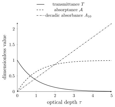
For a pure absorber, $T=e^{-\tau}$, the absorbed fraction is $1-e^{-\tau}$, and $A_{10}=\tau/\ln10$. Absorptance cannot exceed one, whereas absorbance can: $A_{10}=2$ means that $1\%$ of the incident power is transmitted. Reflection and collected scattered light would require a different model.

Cross Sections and Macroscopic Coefficients

Microscopic definition

A cross section is an effective area that converts incident particle or photon flux into an event rate. For one target in a weak incident beam,

$$R_{\mathrm{event}} = \sigma\Phi,$$

where $\Phi$ is the incident number flux in $\mathrm{m^{-2}\,s^{-1}}$. Hence

$$[\sigma]=\mathrm{m^2}.$$

An absorption cross section, scattering cross section, photoionization cross section, and extinction cross section answer different event questions. In electromagnetic energy balance, a passive isolated target obeys

$$\sigma_{\mathrm{ext}} = \sigma_{\mathrm{abs}} + \sigma_{\mathrm{sca}}.$$

Here “absorption” means energy removed from the radiation rather than reradiated; scattering accounts for the reradiated power. Atomic spectroscopy also uses “absorption cross section” for an excitation event, which can later produce fluorescence. Do not count that same excitation once as absorbed power and again as scattered power. Specify which definition is being used.

A gain medium can instead be described by a signed net cross section, but the sign convention and population dependence must then be stated.

Number density and column density

For independent absorbers of number density $n(s)$,

$$\alpha_{\mathrm{abs}}(s) = n(s)\sigma_{\mathrm{abs}}.$$

If the cross section is constant along the path,

$$\tau_{\mathrm{abs}} = \sigma_{\mathrm{abs}}N_{\mathrm{col}},$$

where the column density is

$$N_{\mathrm{col}} = \int n(s)\,ds.$$

The dimensions close:

$$[N_{\mathrm{col}}] = \mathrm{m^{-2}}, \qquad [\sigma N_{\mathrm{col}}] = 1.$$

When multiple species or internal states contribute,

$$\alpha(\nu,s) = \sum_j n_j(s)\sigma_j(\nu).$$

The state populations are part of the model. A database line strength does not by itself specify the cross section of an unequilibrated sample.

Molar absorption coefficients

The common decadic Beer–Lambert form is

$$A_{10} = \varepsilon_{10}c_{\mathrm M}L,$$

where $c_{\mathrm M}$ is molar concentration and the units of $\varepsilon_{10}$ must match those chosen for concentration and path length. A frequently used combination is

$$[\varepsilon_{10}] = \mathrm{L\,mol^{-1}\,cm^{-1}}, \quad [c_{\mathrm M}] = \mathrm{mol\,L^{-1}}, \quad [L] = \mathrm{cm}.$$

For those units, the corresponding effective cross section in $\mathrm{m^2}$ is

$$\sigma_{\mathrm{abs}} = \frac{\ln 10}{10N_{\mathrm A}} \varepsilon_{10}.$$

This is a conversion of the measured coefficient per molecule. Inferring an isolated-molecule oscillator strength from a solution can additionally require solvent and local-field corrections.

The factor $10$ is a unit-conversion factor. It combines litres with cubic metres and centimetres with metres. In coherent SI units, one can instead write

$$\alpha_{\mathrm e} = \kappa_{\mathrm e}c,$$

with $\kappa_{\mathrm e}$ in $\mathrm{m^2\,mol^{-1}}$ and $c$ in $\mathrm{mol\,m^{-3}}$, giving

$$\sigma_{\mathrm{abs}} = \frac{\kappa_{\mathrm e}}{N_{\mathrm A}}.$$

Line-centre and integrated cross sections

A line-centre cross section is a pointwise area:

$$\sigma_0 = \sigma(\nu_0).$$

An integrated cross section includes the chosen spectral coordinate:

$$\Sigma_\nu = \int \sigma(\nu)\,d\nu.$$

Its units are $\mathrm{m^2\,Hz}$, not $\mathrm{m^2}$. An integral over wavenumber or angular frequency has a different numerical value and different units. If

$$\sigma(\nu) = \Sigma_\nu\phi_\nu(\nu),$$

then

$$\int\phi_\nu(\nu)\,d\nu=1,$$

so $\phi_\nu$ has units $\mathrm{Hz^{-1}}$. Never compare a line-centre cross section with an integrated cross section, or two integrated values on different coordinates, without converting the measure.

The Oscillator Strength Reference derives the corresponding integrated-strength relations.

The older phrase extinction coefficient has been used for a linear attenuation coefficient, a molar absorptivity, and the imaginary part of a refractive index. An equation and units make its meaning clear.

Linewidth Nomenclature

A linewidth needs four labels

A reproducible linewidth should specify:

1. the profile or operational estimator;
2. full width, half width, standard deviation, or decay-rate convention;
3. the spectral coordinate and unit; and
4. whether the width is observed, instrument-corrected, homogeneous, inhomogeneous, or model decomposed.

For example, “Gaussian FWHM $\Delta\nu_{\mathrm G}=12.0\,\mathrm{MHz}$ after instrument-response deconvolution” is interpretable. “$\Gamma=12$” is not.

Common width parameters

For a Gaussian profile with standard deviation $\sigma_\nu$,

$$\Delta\nu_{\mathrm{FWHM}}^{(\mathrm G)} = 2\sqrt{2\ln2}\,\sigma_\nu.$$

For a Lorentzian written with HWHM $\gamma_\nu$,

$$L(\nu) \propto \frac{\gamma_\nu} {(\nu-\nu_0)^2+\gamma_\nu^2},$$

the full width is

$$\Delta\nu_{\mathrm{FWHM}}^{(\mathrm L)} = 2\gamma_\nu.$$

A symbol $\Gamma$ may denote either of these widths or an angular-frequency decay rate. The equation defining $\Gamma$ is therefore part of the result.

Label	Meaning	Conversion
Gaussian $\sigma_\nu$	standard deviation	FWHM $=2\sqrt{2\ln2}\,\sigma_\nu$
Lorentzian $\gamma_\nu$	HWHM	FWHM $=2\gamma_\nu$
FWHM	separation of the two half-maximum points	profile dependent
HWHM	half of FWHM for a symmetric profile	FWHM $=2\,\mathrm{HWHM}$
$1/e$ half-width	offset where amplitude or intensity falls to $1/e$	state amplitude versus intensity
decay rate	inverse time constant	relation to spectral width depends on coherence convention

The Line Shape Reference gives the normalized profiles, convolution rules, and lifetime-broadening relations.

Converting widths between coordinates

Frequency, angular frequency, photon energy, and spectroscopic wavenumber are related by constant factors. Their width conversions are exact:

$$\Delta\omega=2\pi\Delta\nu, \qquad \Delta E=h\Delta\nu, \qquad \Delta\tilde\nu=\frac{\Delta\nu}{c}.$$

The last expression uses $\tilde\nu$ in $\mathrm{m^{-1}}$ when $c$ is in $\mathrm{m\,s^{-1}}$. Dividing the numerical result by $100$ gives $\mathrm{cm^{-1}}$.

Wavelength is nonlinear in frequency. For a narrow feature centered at $\lambda_0$, the local approximation is

$$\Delta\lambda_{\mathrm{vac}} \simeq\frac{\lambda_0^2}{c}\Delta\nu.$$

The derivative $d\lambda/d\nu$ is negative, but the width is positive. For a scalar observable such as transmittance, transform the two half-maximum frequencies to obtain the exact wavelength width. For a spectral density, transform the density as well, then find its new maximum and half-maximum points. Those need not be the images of the old points.

Resolving power is a dimensionless instrument or observation metric,

$$\mathcal R = \frac{x_0}{\Delta x},$$

for a declared coordinate and width convention. It is not itself a physical linewidth.

Molecular Branch Notation

Upper and lower state labels

Molecular spectroscopy commonly marks upper-state quantum numbers with a prime and lower-state quantum numbers with a double prime:

$$J' \quad\text{and}\quad J''.$$

Define the branch difference by upper minus lower state,

$$\Delta J = J'-J''.$$

The standard rotational branch letters are:

Branch	$\Delta J$	Upper/lower assignment
O	$-2$	$J'=J''-2$
P	$-1$	$J'=J''-1$
Q	$0$	$J'=J''$
R	$+1$	$J'=J''+1$
S	$+2$	$J'=J''+2$

Which branches are allowed depends on transition type, molecular symmetry, and angular-momentum coupling. The existence of a letter in this table is not a selection rule.

Parenthesized lower-state quantum number

In the common simple-diatomic convention, the integer in a label such as $R(3)$ is the lower-state rotational quantum number:

$$\begin{aligned} R(3):\quad &J''=3\longrightarrow J'=4, \\ P(3):\quad &J''=3\longrightarrow J'=2, \\ Q(3):\quad &J''=3\longrightarrow J'=3. \end{aligned}$$

These upper/lower labels can also be retained for emission: the direction of photon exchange does not by itself reverse the branch letter. Specialized sources may use other conventions, so consult the stated assignments.

A vibronic band is often identified by

$$(v',v''),$$

with upper and lower vibrational quantum numbers in that order. Thus the $(1,0)$ band and the line $R(3)$ within it encode different parts of the assignment.

Multiple angular momenta

Open-shell molecules can carry both rotational angular momentum excluding spin, often $N$, and total angular momentum including spin, $J$. A compound branch label can then encode both

$$\Delta N=N'-N'' \quad\text{and}\quad \Delta J=J'-J''.$$

For example, a source may use a two-letter label in which one letter tracks $\Delta N$ and the other tracks $\Delta J$. Superscripts and subscripts may also identify spin components, parity, $K$, or fine-structure ladders. There is no safe universal decoding rule without the source’s definition.

When a compact label is unfamiliar, start with the explicit upper and lower quantum numbers. See Rotational Spectroscopy and Term Symbol Reference for the underlying angular-momentum labels.

Exercises

Exercise 1: Vacuum and air wavelength

A line has $\lambda_{\mathrm{vac}}=500.000\,\mathrm{nm}$. Using $n_{\mathrm{air}}=1.000277$, find its air wavelength. What happens to its frequency at a stationary vacuum–air interface?

Solution

The air wavelength is

$$\lambda_{\mathrm{air}} = \frac{500.000\ \mathrm{nm}}{1.000277} = 499.862\ \mathrm{nm}.$$

The frequency remains

$$\nu = \frac{c}{\lambda_{\mathrm{vac}}} = 5.99585\times10^{14}\ \mathrm{Hz}.$$

The shorter medium wavelength reflects the smaller phase velocity, not a change in frequency.

Exercise 2: Three attenuation coordinates

A sample has transmittance $T=0.200$. Find the decadic absorbance, Napierian absorbance, and optical depth for a pure-attenuation direct-beam model. If $10\%$ of the incident power is reflected and $15\%$ leaves in an uncollected scattering channel, what is the absorptance?

Solution

The decadic absorbance is

$$A_{10} = -\log_{10}(0.200) = 0.699.$$

The Napierian absorbance is

$$A_{\mathrm e} = -\ln(0.200) = 1.61.$$

Under the stated model,

$$\tau = A_{\mathrm e} = 1.61.$$

The numerical values differ because the logarithm bases differ. With the additional channels, the absorbed fraction is $1-0.200-0.10-0.15=0.55$. Thus $1-T=0.80$ would overestimate absorption. The logarithms of the measured $T$ still have the stated values, but they no longer isolate absorption.

Exercise 3: Molar coefficient to microscopic cross section

A solution has $\varepsilon_{10}=1.50\times10^4\, \mathrm{L\,mol^{-1}\,cm^{-1}}$, concentration $c_{\mathrm M}=20.0\,\mu\mathrm{mol\,L^{-1}}$, and path length $L=1.00\,\mathrm{cm}$. Find $A_{10}$, $T$, $\tau$, and the corresponding microscopic cross section.

Solution

The concentration is

$$c_{\mathrm M} = 2.00\times10^{-5}\ \mathrm{mol\,L^{-1}}.$$

Therefore

$$A_{10} = \varepsilon_{10}c_{\mathrm M}L = 0.300.$$

The transmittance and optical depth are

$$\begin{aligned} T &= 10^{-0.300} = 0.501, \\ \tau &= (\ln10)(0.300) = 0.691. \end{aligned}$$

Using the stated litre–mole–centimetre convention,

$$\begin{aligned} \sigma &= \frac{\ln10}{10N_{\mathrm A}} \varepsilon_{10} \\ &= 5.74\times10^{-21}\ \mathrm{m^2}. \end{aligned}$$

The conversion would change if the numerical value of $\varepsilon$ used a different concentration or length unit.

Exercise 4: Convert a narrow linewidth

A line is centred at $\nu_0=500.0\,\mathrm{THz}$ and has ordinary-frequency FWHM $\Delta\nu=100.0\,\mathrm{MHz}$. Find the central vacuum wavelength and the FWHM in angular frequency and $\mathrm{cm^{-1}}$, and its approximate value in picometres.

Solution

The central wavelength is

$$\lambda_0 = \frac{c}{\nu_0} = 599.6\ \mathrm{nm}.$$

The angular-frequency width is

$$\Delta\omega = 2\pi\Delta\nu = 6.283\times10^8\ \mathrm{rad\,s^{-1}}.$$

The spectroscopic-wavenumber width is

$$\begin{aligned} \Delta\tilde\nu &= \frac{\Delta\nu}{c} \\ &= 0.003336\ \mathrm{cm^{-1}}. \end{aligned}$$

The wavelength width is

$$\begin{aligned} \Delta\lambda &\simeq \frac{\lambda_0^2}{c}\Delta\nu \\ &= 0.1199\ \mathrm{pm}. \end{aligned}$$

Because $\Delta\nu/\nu_0=2.0\times10^{-7}$, the local linear conversion is well justified.

Exercise 5: Decode branch labels

In a simple diatomic absorption spectrum, decode $R(4)$, $P(4)$, and $Q(4)$ in terms of $J''$ and $J'$. Does the notation alone prove all three lines are allowed?

Solution

The parenthesized number labels the lower state:

$$\begin{aligned} R(4):\quad &J''=4,\quad J'=5, \\ P(4):\quad &J''=4,\quad J'=3, \\ Q(4):\quad &J''=4,\quad J'=4. \end{aligned}$$

The labels encode $\Delta J=+1,-1,0$, respectively. They do not prove that the branches are allowed. Electronic symmetry, transition multipolarity, parity, spin, and other angular momenta determine the actual selection rules.

References

• Goenaga-Infante, H., et al. “Glossary of methods and terms used in analytical spectroscopy.” Pure and Applied Chemistry 93, 647–776 (2021). doi:10.1515/pac-2019-0203.
• Hilborn, R. C. “Einstein coefficients, cross sections, $f$ values, dipole moments, and all that.” American Journal of Physics 50, 982–986 (1982). doi:10.1119/1.12937; author’s revised version (2002).
• International Union of Pure and Applied Chemistry. “Absorbance”. Compendium of Chemical Terminology, 5th ed., online version 5.0.0 (2025). Accessed 2026-10-14.
• Kramida, A., Ralchenko, Yu., Reader, J., and NIST ASD Team. “Help for Spectral Lines”. NIST Atomic Spectra Database. Accessed 2026-10-14.
• Schutte, C. J. H., Bertie, J. E., Bunker, P. R., Hougen, J. T., Mills, I. M., Watson, J. K. G., and Winnewisser, B. P. “Notations and conventions in molecular spectroscopy: Part 1. General spectroscopic notation.” Pure and Applied Chemistry 69, 1633–1639 (1997). doi:10.1351/pac199769081633.