Common Atomic Hamiltonians

An atomic Hamiltonian specifies which motions and interactions a model retains. Start with Coulomb binding, then include recoil, relativistic corrections, nuclear spin, and applied fields at the accuracy needed for your question. A small correction to the total binding energy can still strongly mix two nearly degenerate levels.

This reference compares the operators and their regimes of validity. Use the AMO model index to choose the degrees of freedom; follow the subject links below for derivations and spectra. The formulas use SI unless a section explicitly states Hartree units. Angular-momentum operators have units of $\hbar$ in SI; the symbols $I,J,F$ denote their dimensionless quantum numbers.

Helpful background. Atomic units explains how to restore physical units. Familiarity with matrix eigenvalues and perturbation theory helps with the field-dependent examples.

Hydrogenic Hamiltonian

Relative-coordinate form

For one electron and a point nucleus of charge $+Ze$, separation of the center-of-mass motion gives the nonrelativistic relative Hamiltonian

$$H_{\mathrm C} =\frac{\mathbf p^2}{2\mu} -\frac{Ze^2}{4\pi\varepsilon_0r},$$

where

$$\mu =\frac{m_eM}{m_e+M}$$

is the electron–nucleus reduced mass. This model retains Coulomb binding and leading kinematic recoil through $\mu$. It omits relativity, nuclear size, radiative shifts, hyperfine structure, and external fields.

In standard Hartree atomic units,

$$H_{\mathrm C} =-\frac{m_e}{2\mu}\nabla^2-\frac{Z}{r}.$$

For a clamped or infinitely heavy nucleus, $\mu\to m_e$ and

$$H_{\infty} =-\frac12\nabla^2-\frac{Z}{r}.$$

The bound energies of this declared model are

$$E_n =-\frac{\mu}{m_e} \frac{Z^2}{2n^2}E_{\mathrm h}.$$

The Hydrogen Atom page owns the exact bound-state solution. Hydrogen as Atomic Prototype owns the correction ladder needed to compare the ideal model with a measured hydrogen line.

For this spin-independent Coulomb model, $n,\ell,m$ label spatial eigenstates and spin is a spectator. The energy depends only on $n$. A generic central potential preserves rotational symmetry but loses this extra degeneracy between different $\ell$ values.

Multi-Electron Coulomb Hamiltonian

For $N$ nonrelativistic electrons and a clamped point nucleus at the origin, the SI Hamiltonian is

$$H_{\mathrm C} ={} \sum_{i=1}^{N} \left[ \frac{\mathbf p_i^2}{2m_e} -\frac{Ze^2}{4\pi\varepsilon_0r_i} \right] + \sum_{i<j} \frac{e^2}{4\pi\varepsilon_0r_{ij}}.$$

In Hartree atomic units this becomes

$$H_{\mathrm C} ={} \sum_{i=1}^{N} \left( -\frac12\nabla_i^2-\frac{Z}{r_i} \right) +\sum_{i<j}\frac1{r_{ij}}.$$

The physical electronic state belongs to the antisymmetric subspace:

$$P_{ij}\Psi=-\Psi.$$

The electron–electron term couples coordinates, so the exact eigenstate is not generally a single product of one-electron orbitals. The canonical Multi-Electron Atoms chapter develops antisymmetry, shell structure, mean fields, exchange, correlation, and coupling schemes.

Finite nuclear mass

After separating the overall center of mass, a convenient recoil operator contains

$$H_{\mathrm{recoil}}^{(1)} =\frac1{2M} \left( \sum_i\mathbf p_i \right)^2.$$

Expanding the square produces one-electron normal-mass terms and the two-electron mass-polarization term:

$$H_{\mathrm{recoil}}^{(1)} ={} \sum_i\frac{\mathbf p_i^2}{2M} +\frac1M \sum_{i<j} \mathbf p_i\cdot\mathbf p_j.$$

This expression assumes momenta conjugate to electron coordinates relative to the nucleus. Coordinate and sign conventions must be checked before transplanting it into another representation. Precision isotope shifts also contain relativistic recoil, field shifts, and nuclear-polarization effects.

This model excludes relativistic, nuclear-size, radiative, and external-field effects. Separately, a finite basis introduces numerical error even for the chosen Hamiltonian. Johnson (2007) develops the atomic-structure methods used to treat electron correlation and relativistic effects systematically.

Central-Field Reference Hamiltonian

The central-field approximation chooses a separable reference

$$H_0 =\sum_i h_{\mathrm{cf}}(i),$$

with

$$h_{\mathrm{cf}} =-\frac12\nabla^2+V_{\mathrm{cf}}(r)$$

in Hartree units. The exact identity

$$H_{\mathrm C}=H_0+H_{\mathrm{res}}$$

then defines

$$H_{\mathrm{res}} ={} \sum_{i<j}\frac1{r_{ij}} +\sum_i \left[ -\frac{Z}{r_i} -V_{\mathrm{cf}}(r_i) \right].$$

If

$$V_{\mathrm{cf}}(r) =-\frac{Z}{r}+U(r),$$

the residual simplifies to

$$H_{\mathrm{res}} =\sum_{i<j}\frac1{r_{ij}} -\sum_iU(r_i).$$

The subtraction is essential: once an average interaction $U$ has been added to $H_0$, it must be removed from the residual before the full electron–electron interaction is restored.

Meaning of the reference

A local central field guarantees

$$[h_{\mathrm{cf}},L^2]=0, \qquad [h_{\mathrm{cf}},L_z]=0,$$

and orbitals can be labeled by $n,\ell,m$. It does not guarantee hydrogenic degeneracy between different $\ell$, nor does it make orbital energies equal to exact ionization or excitation energies.

A local fitted potential, a Hartree electrostatic field, and a Hartree–Fock operator are different approximations: exchange makes the last generally nonlocal. Similar orbital labels do not make their eigenvalues equivalent to measured ionization energies. See Central-field approximation for screening and self-consistency.

Fine-Structure Operators

One-electron Pauli correction

For a spin-$1/2$ electron in a static central potential energy $V(r)$, the nonrelativistic reference is

$$H_0 =\frac{\mathbf p^2}{2m_e}+V(r).$$

The Foldy–Wouthuysen expansion gives, through order $1/c^2$, the leading one-electron correction

$$H_{\mathrm{fs}}^{(1)} =H_{\mathrm{mv}}+H_{\mathrm{so}}+H_D,$$

with

$$H_{\mathrm{mv}} =-\frac{\mathbf p^4}{8m_e^3c^2},$$ $$H_{\mathrm{so}} =\frac1{2m_e^2c^2} \frac1r\frac{dV}{dr} \mathbf L\cdot\mathbf S,$$

and

$$H_D =\frac{\hbar^2}{8m_e^2c^2} \nabla^2V.$$

$H_{\mathrm{mv}}$ is the relativistic kinetic correction, $H_{\mathrm{so}}$ is the spin–orbit term including the Thomas factor, and $H_D$ is the Darwin term. Spin–orbit coupling is therefore one part of fine structure, not a synonym for the entire correction.

In Hartree atomic units, $c=\alpha^{-1}$ and the same terms become

$$\begin{aligned} H_{\mathrm{mv}} &=-\frac{\alpha^2}{8}\mathbf p^4,\\ H_{\mathrm{so}} &=\frac{\alpha^2}{2r} \frac{dV}{dr} \mathbf L\cdot\mathbf S,\\ H_D &=\frac{\alpha^2}{8}\nabla^2V. \end{aligned}$$

Here angular momenta and momenta are represented in their Hartree-unit numerical form with $\hbar=1$.

Treat these as low-momentum effective corrections, normally evaluated perturbatively. The truncated kinetic energy $p^2/(2m_e)-p^4/(8m_e^3c^2)$ tends to $-\infty$ as $p\to\infty$; minimizing it over unrestricted momenta is not a valid relativistic theory.

Point-Coulomb spin–orbit term

For

$$V(r) =-\frac{Ze^2}{4\pi\varepsilon_0r},$$

the SI spin–orbit operator is

$$H_{\mathrm{so}} = \frac{Ze^2} {8\pi\varepsilon_0m_e^2c^2r^3} \mathbf L\cdot\mathbf S.$$

The angular identity

$$2\mathbf L\cdot\mathbf S =J^2-L^2-S^2$$

diagonalizes this operator in a fixed $\ell,s,j$ manifold. A rotationally invariant spin–orbit interaction preserves $J,m_J$ and parity, while $L$ and $S$ can cease to be exact in general many-electron intermediate coupling.

Multi-electron boundary

Many-electron fine structure can also contain spin–other-orbit, mutual spin–orbit, spin–spin, and orbit–orbit terms, or be described from a Dirac–Coulomb–Breit baseline. The one-electron Pauli form is controlled when momenta are nonrelativistic and $Z\alpha\ll1$. Heavy highly charged ions require a relativistic starting point rather than an uncontrolled sequence of low-order patches.

Fine Structure develops the derivation, hydrogenic spectrum, many-electron coupling, and boundaries of the expansion.

Zeeman Hamiltonians

Linear magnetic coupling

For a static field $\mathbf B$, a common leading energy Hamiltonian is

$$H_Z =\frac{\mu_{\mathrm B}}{\hbar} \left( g_L\mathbf L +g_S\mathbf S +g_I'\mathbf I \right) \cdot\mathbf B.$$

The electronic coefficients $g_L$ and $g_S$ are positive in this energy convention; the negative electron charge is already included in $-\boldsymbol\mu\cdot\mathbf B$. The nuclear coefficient

$$g_I' =-g_I\frac{\mu_{\mathrm N}}{\mu_{\mathrm B}}$$

is defined on the Bohr-magneton scale. Confusing it with the nuclear $g$ factor paired with $\mu_{\mathrm N}$ introduces a factor near $m_p/m_e$ and can reverse a sign.

If $\mathbf B=B\hat{\mathbf z}$ and fine structure is dominant over the magnetic interaction, projection into an isolated $J$ level gives

$$\Delta E =g_J\mu_{\mathrm B}m_JB.$$

If hyperfine coupling is also dominant over the magnetic interaction, projection into an isolated $F$ manifold gives

$$\Delta E =g_F\mu_{\mathrm B}m_FB.$$

These are first-order effective formulas, not replacements for the operator when the field mixes $J$ or $F$ manifolds.

Diamagnetic term

For a uniform field in the symmetric gauge,

$$\mathbf A =\frac12\mathbf B\times\mathbf r,$$

minimal coupling produces the one-electron diamagnetic term

$$H_{\mathrm{dia}} =\frac{e^2}{8m_e} \lvert\mathbf B\times\mathbf r\rvert^2.$$

It is quadratic in $B$. Second-order level shifts also arise from virtual mixing by the linear Zeeman operator. These are distinct contributions and must be combined consistently.

Field-regime test

The word “weak” is relative to a particular zero-field splitting:

Comparison	Useful labels	Treatment
$\mu_{\mathrm B}B\ll\Delta E_{\mathrm{hfs}}$	$F,m_F$	projected $g_F$ formula
$\mu_{\mathrm B}B\sim\Delta E_{\mathrm{hfs}}$	$m_F$ exact, $F$ mixed	diagonalize fixed-$m_F$ blocks
$\Delta E_{\mathrm{hfs}}\ll\mu_{\mathrm B}B\ll\Delta E_{\mathrm{fs}}$	$m_I,m_J$	hyperfine Paschen–Back basis
$\mu_{\mathrm B}B\sim\Delta E_{\mathrm{fs}}$	total axial projection	include neighboring $J$ levels

Zeeman Effect in Atoms develops Landé factors, Breit–Rabi crossover spectra, Paschen–Back regimes, polarization-resolved transitions, and experimental interpretation.

Stark Hamiltonians

Uniform electric field

In the long-wavelength electric-dipole approximation,

$$H_E(t) =-\mathbf d\cdot\boldsymbol{\mathcal E}(t),$$

where the total dipole operator is

$$\mathbf d=\sum_a q_a\mathbf r_a$$

relative to a declared origin. For one electron relative to a fixed nucleus,

$$\mathbf d=-e\mathbf r.$$

For a neutral atom the total internal dipole is independent of an overall origin shift. For an ion it is not: separate center-of-mass and internal coordinates before interpreting a uniform-field coupling, and state which motion the model retains.

For a static field $\boldsymbol{\mathcal E}=\mathcal E\hat{\mathbf z}$,

$$H_E=-\mathcal E d_z.$$

The dipole approximation requires the field to vary little over the atomic size. Field gradients introduce quadrupole and higher-multipole couplings.

Perturbative scale

For a state $|a\rangle$ coupled to $|b\rangle$, define

$$\eta_{ab} = \frac{ \mathcal E \lvert\langle a|d_z|b\rangle\rvert }{ \lvert E_a^{(0)}-E_b^{(0)}\rvert }.$$

A large $\eta_{ab}$ identifies a state that must be included explicitly. Small individual ratios are only a first check: many weakly coupled states can have a substantial combined effect. For a nondegenerate state, the first-order admixture has squared norm $\sum_{b\ne a}\eta_{ab}^2$; this sum must also be small for the state correction to be small. Near a degeneracy, diagonalize the coupled manifold before expanding.

For an isolated nondegenerate parity eigenstate, the leading static shift is usually

$$\Delta E_a =-\frac12\alpha_a(0)\mathcal E^2.$$

This is a derived effective energy after virtual opposite-parity states have been eliminated. It is not an additional microscopic interaction to add on top of an explicit dipole-coupled basis, or the same mixing is counted twice.

For two opposite-parity levels separated by $\delta$, choose phases so that the dipole matrix element $d$ is real. The projected Hamiltonian

$$H_{\mathrm{eff}} = \begin{pmatrix} -\delta/2 & -d\mathcal E\\ -d\mathcal E & \delta/2 \end{pmatrix}$$

has a linear splitting when $\delta=0$. Thus parity symmetry does not forbid the linear Stark effect inside a degenerate manifold.

Stark Effect in Atoms develops static and dynamic polarizability, hydrogenic degeneracy, scalar/vector/tensor responses, magic conditions, and experimental field calibration.

Hyperfine Hamiltonians

Foot (2005) develops these angular-momentum models and their spectroscopic interpretation.

Hyperfine structure couples nuclear electromagnetic multipoles to electronic fields at the nucleus. A rotationally invariant expansion is

$$H_{\mathrm{hfs}} =\sum_{k\ge1} T_{\mathrm{nuc}}^{(k)} \cdot T_{\mathrm{el}}^{(k)}.$$

The leading $k=1$ term is magnetic dipole; $k=2$ is electric quadrupole.

Magnetic-dipole term

Within an isolated electronic level of angular momentum $J$,

$$H_{\mathrm{M1}} =\frac{A}{\hbar^2} \mathbf I\cdot\mathbf J.$$

With

$$\mathbf F=\mathbf I+\mathbf J$$

and

$$K =F(F+1)-I(I+1)-J(J+1),$$

the first-order energy is

$$E_F^{\mathrm{M1}} =\frac A2K.$$

$A$ includes both the nuclear magnetic moment and the electronic magnetic field at the nucleus. It can be positive or negative and is state- and isotope-specific.

Electric-quadrupole term

For $I\ge1$ and $J\ge1$, the conventional first-order quadrupole energy is

$$\begin{aligned} E_F^{\mathrm{E2}} &=B\frac{N_{IJF}}{D_{IJ}},\\ N_{IJF} &=\frac34K(K+1) -I(I+1)J(J+1),\\ D_{IJ} &=2I(2I-1)J(2J-1). \end{aligned}$$

The standard dipole-plus-quadrupole model is

$$E_F^{\mathrm{hfs}} =\frac A2K+E_F^{\mathrm{E2}}.$$

For $I<1$ or $J<1$, the first-order $B$ term is absent. Databases often quote $A/h$ and $B/h$ in MHz while labeling the columns simply $A$ and $B$. Determine whether the constants are energies or frequencies before using them.

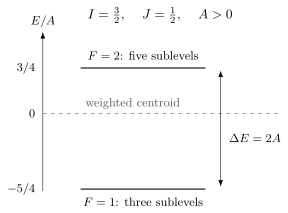
For $I=3/2$, $J=1/2$, and $A>0$, the two hyperfine levels lie at $-5A/4$ and $3A/4$. Their separation is $2A$, and weighting each by its $2F+1$ magnetic sublevels leaves the centroid unchanged. The exercise below derives these numbers.

Hyperfine plus magnetic field

When the Zeeman energy is not small compared with hyperfine intervals, use

$$H =H_{\mathrm{hfs}}+H_Z$$

and diagonalize in a basis such as $|I,m_I\rangle|\gamma,J,m_J\rangle$ at fixed axial projection. Substituting a field-dependent $g_F$ into a weak-field formula is not equivalent.

Hyperfine Structure develops the microscopic interactions, interval rules, hydrogen and alkali examples, clock transitions, and field crossovers.

Rydberg Interaction Models

Saffman, Walker, and Mølmer (2010) review these pair-state and driven-array reductions. Rydberg interactions are effective atomic Hamiltonians obtained after choosing asymptotic pair states, multipole order, geometry, and external fields.

Dipole–dipole operator

At separation $R$ much larger than the electronic-cloud size, but small compared with $c/\omega$, where $\omega$ is the angular frequency of the relevant dipole transition, the leading nonretarded electric dipole–dipole operator is

$$V_{dd}(\mathbf R) ={} \frac1{4\pi\varepsilon_0R^3} \left[ \mathbf d_1\cdot\mathbf d_2 -3(\mathbf d_1\cdot\hat{\mathbf R}) (\mathbf d_2\cdot\hat{\mathbf R}) \right].$$

It is an anisotropic operator in the magnetic-sublevel pair space, not a universal scalar potential.

Two-channel pair Hamiltonian

If a prepared pair state $|rr\rangle$ couples mainly to $|r'r''\rangle$, subtract the energy of $|rr\rangle$ and write

$$H_{\mathrm{pair}} = \begin{pmatrix} 0 & V_{dd}\\ V_{dd}^* & \Delta_F \end{pmatrix},$$

where

$$\Delta_F =E_{r'}+E_{r''}-2E_r$$

is the Förster defect.

For

$$\lvert V_{dd}\rvert\ll\lvert\Delta_F\rvert,$$

the shift of the prepared channel is

$$\Delta E_{rr} \simeq-\frac{\lvert V_{dd}\rvert^2}{\Delta_F} =\frac{C_6}{R^6}.$$

The sign of $C_6$ follows from the channel defects and matrix elements. Near resonance,

$$\lvert\Delta_F\rvert \lesssim \lvert V_{dd}\rvert,$$

the channels must be diagonalized and the leading splitting scales as $C_3/R^3$.

Driven two-level array

After selecting one ground state $|g_i\rangle$ and one Rydberg state $|r_i\rangle$, transforming to a rotating frame, and adopting the rotating- wave approximation, a common coherent array model is

$$\frac H\hbar ={} \sum_i \frac{\Omega_i}{2} \left( e^{i\phi_i}|r_i\rangle\langle g_i| +\mathrm{h.c.} \right) -\sum_i\Delta_i n_i +\sum_{i<j} \frac{V_{ij}}{\hbar}n_in_j,$$

with

$$n_i=|r_i\rangle\langle r_i|.$$

The sign shown uses

$$\Delta_i=\omega_{L,i}-\omega_{rg,i}.$$

Some sources define the opposite detuning. The drive amplitude may also be defined with or without the factor $1/2$.

This model omits leakage levels, intermediate-state scattering, motion, position-dependent phases, state-changing pair interactions, dissipation, and readout error unless those are added explicitly. Rydberg Atoms Basics develops the scaling and pair-channel physics; Rydberg Blockade develops finite-blockade dynamics and projected many-body limits.

Perturb or Diagonalize?

The important question is not whether a correction “looks small” in absolute units, but whether its matrix elements are small relative to the energy denominators connecting retained and omitted states.

Let $P$ project onto a chosen model space and $Q=1-P$. Eliminating the $Q$ component of the stationary Schrödinger equation gives the exact energy-dependent operator, wherever the resolvent exists,

$$H_{\mathrm{eff}}(E) ={}PHP +PHQ \frac1{E-QHQ} QHP.$$

Small denominators or a large combined coupling to $Q$ prevent a simple low-order expansion. In a finite or otherwise well-controlled model space, compare the norm of the coupling block $QHP$ with the separation from the relevant $QHQ$ spectrum. A global norm of an unbounded Coulomb or position operator is not a useful substitute for that restricted comparison.

For example, let one state of energy zero couple with amplitude $v$ to each of $N$ degenerate states of energy $\Delta>0$. Only their normalized symmetric combination couples to it, with matrix element $\sqrt N v$. Every pairwise ratio $|v|/\Delta$ may be small while $\sqrt N|v|/\Delta$ is not. The last exercise quantifies the resulting mixing.

The same elimination produces quadratic Stark energies and off-resonant Rydberg pair shifts. Enlarge the retained space around an avoided crossing; near a continuum threshold, a discrete finite matrix may also miss decay or resonance behavior. See Effective Hamiltonians.

Symmetry and Good-Label Table

“Good quantum number” means that the declared Hamiltonian commutes with the corresponding observable and that the relevant eigenvalue distinguishes the states under discussion.

Declared model	Typically exact labels or sectors	Labels that may fail
one-electron Coulomb, no spin terms	$\ell,m$, parity; $n$ labels bound energy	fine-, hyperfine-, and field-dressed labels absent
spin-independent multi-electron Coulomb	$L,S,M_L,M_S$, or the coupled choice $L,S,J,M_J$; parity	configurations and orbital occupations need not be exact
local central field	one-electron $\ell,m$ and parity	hydrogenic degeneracy across $\ell$
rotationally invariant fine structure	total $J,m_J$, parity	separate $L,S$ in intermediate coupling
zero-field hyperfine	$F,m_F$, parity	separate $m_I,m_J$
uniform dc electric field along $z$	axial projection $m$	parity and usually total angular-momentum magnitude
uniform dc magnetic field along $z$	axial total projection and parity	$F$ or $J$ across Paschen–Back crossovers
crossed nonparallel electric and magnetic fields	only surviving discrete symmetries, if any	a universal magnetic projection
axial Rydberg pair problem	total axial projection and exchange sectors when applicable	individual atomic $m$ under anisotropic mixing

The uncoupled and coupled angular-momentum sets in the second row are alternative compatible choices; $J^2,L_z,S_z$ cannot generally be diagonalized together. Degeneracy alone does not imply a symmetry label, and a familiar label can remain useful approximately after it ceases to be exact. Report dominant components or expectation values when assigning mixed states.

Units, Gauges, and Frames

Energy versus frequency Hamiltonians

Some AMO literature writes $H$ in energy units; other literature writes $H/\hbar$ in angular-frequency units. These equations are not numerically identical:

$$i\hbar\frac{d}{dt}|\psi\rangle =H|\psi\rangle$$

becomes

$$i\frac{d}{dt}|\psi\rangle =\frac H\hbar|\psi\rangle.$$

A matrix entry labeled “MHz” may mean $H/h$ in cycles per second or $H/\hbar$ with a convention that quotes $\Omega/(2\pi)$. State the defining equation.

The Atomic Units reference gives the Hartree conversion and dimensional restoration rules.

Length and velocity gauges

For a time-dependent electromagnetic field, the dipole coupling

$$-\mathbf d\cdot\boldsymbol{\mathcal E}(t)$$

is a length-gauge form. A minimal-coupling or velocity-gauge Hamiltonian uses $\mathbf p-q\mathbf A$. The formulations are related by a unitary gauge transformation in a complete, consistently transformed theory. Inconsistent basis truncations or observables can break numerical gauge agreement. The $A^2$ term must be treated consistently: for a prescribed spatially uniform classical vector potential its contribution is a time-dependent scalar and can be removed by a global phase. That simplification does not apply generally to spatially varying or quantized fields.

Do not add a length-gauge dipole term and a velocity-gauge $\mathbf p\cdot\mathbf A$ term for the same field unless a derivation explicitly requires both.

Rotating frames

For the state convention $|\psi_{\mathrm{rot}}\rangle=U(t)|\psi\rangle$, a rotating-frame transformation changes the Hamiltonian by

$$H_{\mathrm{rot}} =UHU^\dagger +i\hbar\dot U U^\dagger.$$

The second term generates detunings and frame-dependent energy zeros. A rotating-wave approximation is an additional step that discards rapidly oscillating terms. Specify the sign of detuning and whether the quoted drive is $\Omega$ or $\Omega/(2\pi)$; transform observables along with states.

Common pitfalls

Adding the same response twice. A fitted potential may already include core polarization or relativistic shifts. Likewise, the quadratic Stark energy is generated by virtual dipole transitions; add a separate polarizability only for channels absent from the explicit model.

Keeping weak-field labels through a crossover. When fields mix levels, the old $F$ or $J$ values become approximate labels. Use exact symmetry blocks and inspect the eigenvectors. Stretched states can remain unmixed even when other sublevels mix strongly.

Confusing levels with spectral lines. A transition frequency is an energy difference. Its strength also needs a transition matrix element and the preparation and detection conditions. A basis orbital energy alone is usually neither quantity.

Exercises

Central-field subtraction

Let

$$V_{\mathrm{cf}}(r) =-\frac Zr+U(r).$$

Starting from the many-electron Coulomb Hamiltonian, derive the residual interaction associated with

$$H_0=\sum_i \left[ -\frac12\nabla_i^2+V_{\mathrm{cf}}(r_i) \right].$$

Solution

The full Coulomb Hamiltonian is

$$H_{\mathrm C} =\sum_i \left( -\frac12\nabla_i^2-\frac Z{r_i} \right) +\sum_{i<j}\frac1{r_{ij}}.$$

Subtracting $H_0$ gives

$$\begin{aligned} H_{\mathrm{res}} &=H_{\mathrm C}-H_0,\\ &=\sum_{i<j}\frac1{r_{ij}} -\sum_iU(r_i). \end{aligned}$$

The second term removes the average interaction already inserted into the reference. Keeping the full pair repulsion without this counterterm would count the reference field twice.

Choose a Zeeman treatment

An alkali ground state has a hyperfine interval $\Delta E_{\mathrm{hfs}}/h=6.8\ \mathrm{GHz}$. At a given field, $\mu_{\mathrm B}B/h=4.0\ \mathrm{GHz}$, while the nearest fine-structure interval is hundreds of terahertz. Should one use a fixed-$F$ Landé formula, an uncoupled electronic fine-structure calculation, or another treatment?

Solution

The magnetic energy is comparable to the hyperfine interval:

$$\frac{\mu_{\mathrm B}B} {\Delta E_{\mathrm{hfs}}} \approx0.59.$$

This scale does not justify a fixed-$F$ first-order formula for general sublevels. Mixing depends on $m_F$ and the actual Zeeman matrix elements; stretched states remain unmixed within this isolated-$J$ model. The field is still tiny compared with the fine-structure interval, so one can keep the isolated electronic $J$ level and diagonalize

$$H_{\mathrm{hfs}}+H_Z$$

in fixed-$m_F$ blocks, for example in the $|I,m_I\rangle|J,m_J\rangle$ basis. There is no need to mix remote fine-structure levels at this scale unless the desired precision exposes their second-order contribution.

Stark shift without double counting

A truncated basis explicitly contains $|g\rangle$ and several opposite-parity excited states, coupled by $-\mathbf d\cdot\boldsymbol{\mathcal E}$. A second model term $-\alpha_g\mathcal E^2/2$ is then added to $|g\rangle$. Under what condition is this likely double counting?

Solution

The second-order shift generated by the explicit dipole coupling is

$$\Delta E_g^{(2)} = \sum_{n\ne g} \frac{ \lvert\langle n|d_z|g\rangle\rvert^2 \mathcal E^2 }{ E_g-E_n }.$$

If $\alpha_g$ was computed from the same excited states and matrix elements, then adding $-\alpha_g\mathcal E^2/2$ counts their virtual response a second time. An extra effective polarizability term is justified only for channels excluded from the explicit basis, with a declared subtraction or partition showing which contribution it represents.

Hyperfine splitting and its centroid

For $I=3/2,J=1/2$, find the magnetic-dipole hyperfine energies and check their degeneracy-weighted centroid. Can the first-order quadrupole constant $B$ shift these levels?

Solution

The allowed values are $F=1,2$. Substitution into $K$ gives $K_1=-5/2$ and $K_2=3/2$, hence

$$E_1=-5A/4,\qquad E_2=3A/4.$$

There are $2F+1=3,5$ magnetic sublevels, so

$$\frac{3E_1+5E_2}{8}=0,\qquad E_2-E_1=2A.$$

The electronic $J=1/2$ level has no diagonal rank-2 tensor, so the first-order quadrupole term vanishes, even if the nucleus has a quadrupole moment. Higher-order mixing with other electronic levels is a separate effect.

Many small couplings

One state $|a\rangle$ has energy zero and couples with real amplitude $v$ to each of $N$ mutually uncoupled states $|b_j\rangle$ of energy $\Delta>0$. Find the weight outside $|a\rangle$ in the lower eigenstate. Evaluate it for $v/\Delta=0.01$ and $N=10^4$. Does checking each pair separately suffice?

Solution

The bright combination $|B\rangle=N^{-1/2}\sum_j|b_j\rangle$ has coupling $\sqrt N v$; the other $N-1$ combinations decouple. Diagonalize

$$H_{aB}=\begin{pmatrix}0&\sqrt N v\\ \sqrt N v&\Delta\end{pmatrix}.$$

The lower eigenvector has omitted-space probability

$$P_B=\frac12\left(1-\frac{\Delta}{\sqrt{\Delta^2+4Nv^2}}\right).$$

For small $Nv^2/\Delta^2$, this is $Nv^2/\Delta^2$, the sum of the first-order admixture probabilities. Here $Nv^2/\Delta^2=1$, so the exact weight is $(1-1/\sqrt5)/2\simeq0.2764$. Individual couplings of one percent do not guarantee a small total change of state.

References

• Foldy, L. L., and S. A. Wouthuysen. “On the Dirac Theory of Spin 1/2 Particles and Its Non-Relativistic Limit.” Physical Review 78, 29–36 (1950). DOI.
• Foot, C. J. Atomic Physics. Oxford University Press, 2005. Publisher.
• Johnson, W. R. Atomic Structure Theory: Lectures on Atomic Physics. Springer, 2007. DOI.
• Saffman, M., T. G. Walker, and K. Mølmer. “Quantum information with Rydberg atoms.” Reviews of Modern Physics 82, 2313–2363 (2010). DOI.