Oscillator Strength Reference

An oscillator strength is a dimensionless, energy-weighted measure of an electric-dipole transition. It is useful precisely because the same number can connect a structure calculation, an integrated absorption measurement, and a radiative transition probability. That portability is lost if the averaging, degeneracy, line grouping, or spectral coordinate is left implicit.

Here $f$ means an electric-dipole (E1) absorption oscillator strength. A value for one magnetic substate, a fine-structure level, and a whole molecular band can represent different averages and sums. The formulas below specify those choices before connecting $f$ to dipole moments, radiative rates, and absorption areas.

Helpful background. Oscillator Strengths explains why transition energies weight dipole matrix elements and derives the sum rule.

Oscillator strengths and transition labels

Throughout the main formulas:

• $i$ is the lower state or level and $f$ is the upper state or level;
• $\Delta E=E_f-E_i>0$ and $\omega_{fi}=\Delta E/\hbar>0$;
• $f_{if}>0$ is an absorption oscillator strength;
• $g_i$ and $g_f$ are the statistical weights of the lower and upper objects;
• $\widehat{\mathbf D}$ includes electric charge and has SI units $\mathrm{C\,m}$;
• $\widehat{\mathbf R}=\widehat{\mathbf D}/(-e)$ is the corresponding charge-free electronic position operator when that notation is useful;
• $S_{if}$ is an E1 reduced line strength, with its angular-momentum convention stated below; and
• line profiles are normalized to unit area in the spectral coordinate printed in their subscript.

The electron charge is $-e$, where $e>0$. A sign change in the dipole operator does not affect a strength because the matrix element is squared.

Dipole matrix elements

Polarization-resolved state-to-state strength

For specified stationary states and a unit, possibly complex polarization vector $\boldsymbol{\epsilon}$, define the absorption field convention by $\mathbf E^{(+)}\propto\boldsymbol{\epsilon}e^{-i\omega t}$. The absorption matrix element is $\langle f|\widehat{\mathbf D}\cdot\boldsymbol{\epsilon}|i\rangle$, giving

$$f_{if}^{(\epsilon)} = \frac{2m_e\omega_{fi}} {\hbar e^2} \left| \boldsymbol{\epsilon}\mathbin{\cdot} \langle f|\widehat{\mathbf D}|i\rangle \right|^2.$$

This quantity describes the selected field component. It should not be averaged over three polarizations a second time.

Isotropic state-to-state strength

For an isotropic average over three orthogonal field directions,

$$\begin{aligned} f_{if} &= \frac{1}{3} \sum_{\alpha=x,y,z} f_{if}^{(\alpha)} \\ &= \frac{2m_e\omega_{fi}} {3\hbar e^2} \left| \langle f|\widehat{\mathbf D}|i\rangle \right|^2. \end{aligned}$$

Equivalently, using the charge-free position operator,

$$f_{if} = \frac{2m_e\Delta E} {3\hbar^2} \left| \langle f|\widehat{\mathbf R}|i\rangle \right|^2.$$

The factor $1/3$ is a polarization or orientation average. It is not a universal factor for every resolved experiment.

Level-averaged reduced strength

For atomic fine-structure levels, define the reduced E1 line strength

$$S_{if} = \left| \left\langle \gamma_fJ_f \left\| \widehat{\mathbf D}^{(1)} \right\| \gamma_iJ_i \right\rangle \right|^2.$$

Use the following Wigner–Eckart convention:

$$\langle\gamma_fJ_fM_f|D_q|\gamma_iJ_iM_i\rangle =(-1)^{J_f-M_f} \begin{pmatrix}J_f&1&J_i\\-M_f&q&M_i\end{pmatrix} \times\langle\gamma_fJ_f\|D^{(1)}\|\gamma_iJ_i\rangle.$$

Summing squared matrix elements over $M_i,M_f,q$ gives $S_{if}$. An isotropic Cartesian average then contributes $1/3$, while equal populations of the initial magnetic substates contribute $1/g_i$, with $g_i=2J_i+1$. Thus

$$f_{if} = \frac{2m_e\omega_{fi}} {3\hbar e^2g_i} S_{if}.$$

For an unpolarized lower level in a rotationally invariant atom, the response summed over final substates is independent of the direction of a normalized incident polarization. The expression above therefore describes that experiment too. It is not a sum over three independent physical photon polarizations: a plane wave has two transverse polarizations. Prepared magnetic substates require the resolved formula.

Atomic-unit form

When $\Delta E$ is in hartrees and $S_{if}$ is in $e^2a_0^2$,

$$f_{if} = \frac{2}{3} \frac{\Delta E}{g_i} S_{if}.$$

For nondegenerate states with $R_{if}=|\langle f|\widehat{\mathbf R}|i\rangle|$ in $a_0$,

$$f_{if} = \frac{2}{3} \Delta E\,R_{if}^2.$$

“Atomic units” must apply to both the transition energy and the matrix element. Inserting an energy in electronvolts into either formula gives a dimensionless but incorrect result.

Strength quantities at a glance

Symbol	Definition in this reference	Units
$f_{if}$	E1 absorption oscillator strength	dimensionless
$g_if_{if}$ or $gf$	weighted absorption oscillator strength	dimensionless
$\log(gf)$	$\log_{10}(g_if_{if})$	dimensionless
$S_{if}$	squared reduced E1 matrix element	$\mathrm{C^2\,m^2}$ or $e^2a_0^2$
$A_{fi}$	spontaneous-emission probability per unit time	$\mathrm{s^{-1}}$
$\mathbf D_{fi}$	transition dipole including charge	$\mathrm{C\,m}$ or $ea_0$
$\int\sigma_\nu\,d\nu$	frequency-integrated absorption cross section	$\mathrm{m^2\,Hz}$

Three distinctions prevent most conversion errors:

1. $f$ and $gf$ are not the same number.
2. $A_{fi}$ runs from the upper object to the lower object, whereas $f_{if}$ is conventionally an absorption strength.
3. $S$ contains the matrix element but no explicit frequency factor. At fixed $S$, $f\propto\omega$ and $A\propto\omega^3$. Changing the Hamiltonian generally changes the wavefunctions and hence $S$ as well.

Direct Conversion Formulas

Weighted strength and logarithmic strength

$$gf = g_i f_{if}, \qquad \log(gf) = \log_{10}\!\left(g_i f_{if}\right).$$

The logarithm is base ten. Recovering $f$ requires both the quoted logarithm and the lower statistical weight:

$$f_{if} = \frac{10^{\log(gf)}}{g_i}.$$

Absorption strength and spontaneous rate

For an E1 transition in free space, using the same level definitions for both strengths (Hilborn 2002),

$$A_{fi} = \frac{e^2\omega_{fi}^{\,2}} {2\pi\epsilon_0m_ec^3} \frac{g_i}{g_f} f_{if}.$$

Equivalently,

$$f_{if} = \frac{2\pi\epsilon_0m_ec^3} {e^2\omega_{fi}^{\,2}} \frac{g_f}{g_i} A_{fi}.$$

In wavelength form,

$$A_{fi} = \frac{2\pi e^2} {\epsilon_0m_ec\lambda^2} \frac{g_i}{g_f} f_{if}.$$

The vacuum wavelength $\lambda=2\pi c/\omega_{fi}$ must be used in this relation. Air wavelengths can matter at the precision level of critically evaluated spectroscopy.

NIST-style numerical forms

For $\lambda$ in ångströms and $A_{fi}$ in $\mathrm{s^{-1}}$,

$$f_{if} = 1.49919\times10^{-16} \frac{g_f}{g_i} \lambda_{\mathring{\mathrm A}}^{\,2} A_{fi}.$$

The corresponding weighted form is

$$g_i f_{if} = 1.49919\times10^{-16} g_f\lambda_{\mathring{\mathrm A}}^{\,2}A_{fi}.$$

If a table prints $A$ in units of $10^8\,\mathrm{s^{-1}}$, replace the coefficient $10^{-16}$ by $10^{-8}$. Mixing those two column conventions creates an error of eight orders of magnitude.

For $S_{if}$ in atomic units,

$$A_{fi} = \frac{2.02613\times10^{18}} {g_f\lambda_{\mathring{\mathrm A}}^{\,3}} S_{if},$$

and

$$g_i f_{if} = \frac{303.756} {\lambda_{\mathring{\mathrm A}}} S_{if}.$$

These NIST numerical forms assume an E1 reduced line strength in $e^2a_0^2$. Different multipoles use different dimensions and wavelength powers.

Reverse and signed strengths

If the same algebraic convention is extended to the reverse transition, $\omega_{if}<0$ and

$$g_i f_{if} = -g_f f_{fi}.$$

Thus an absorption strength is positive and its signed downward counterpart is negative. Some tables instead quote only positive magnitudes for both directions. Never infer the sign convention from subscripts alone.

Integrated Absorption

An oscillator strength controls the area of a weak, isolated absorption line, not its peak height. Let $L_\nu(\nu)$ be normalized by

$$\int_{-\infty}^{\infty} L_\nu(\nu)\,d\nu = 1.$$

Then

$$\sigma_\nu(\nu) = \frac{e^2} {4\epsilon_0m_ec} f_{if}L_\nu(\nu),$$

so

$$\int_{-\infty}^{\infty} \sigma_\nu(\nu)\,d\nu = \frac{e^2} {4\epsilon_0m_ec} f_{if}.$$

Numerically,

$$\frac{e^2} {4\epsilon_0m_ec} = 2.6540\times10^{-6} \ \mathrm{m^2\,Hz}.$$

This is the weak-probe cross section per atom initially in the specified lower level, with negligible upper population and no saturation or interfering neighboring transition. Redistribution among line frequencies preserves its area under this model. Optical thinness is needed to identify fractional power loss directly with column density times cross section; the cross section itself can also be used in the exponential Beer–Lambert law for an optically thick sample in linear response.

Angular-frequency axis

The monochromatic cross section is the same at the same photon energy: $\sigma_\omega(\omega)=\sigma_\nu(\omega/2\pi)$. It is not a density per unit frequency. The normalized profile does transform as a density, $L_\omega(\omega)=L_\nu(\omega/2\pi)/(2\pi)$. Therefore

$$\int \sigma_\omega(\omega)\,d\omega = \frac{\pi e^2} {2\epsilon_0m_ec} f_{if}.$$

The angular-frequency area is $2\pi$ times the ordinary-frequency area because the integration measure changed while the cross section did not. Use the corresponding area coefficient with each normalized profile. The distinction is illustrated in the Line Shape Reference.

Spectroscopic-wavenumber axis

For $\widetilde\nu=\nu/c$ in inverse metres,

$$\int \sigma_{\widetilde\nu}(\widetilde\nu) \,d\widetilde\nu = \frac{e^2} {4\epsilon_0m_ec^2} f_{if}.$$

If the wavenumber is reported in $\mathrm{cm^{-1}}$, the profile and integration measure must use that same unit.

Decadic molar absorption coefficient

For an isotropic dilute sample in the same weak-probe, electric-dipole convention, molecular spectroscopy often reports a decadic molar absorption coefficient $\epsilon(\widetilde\nu)$ in $\mathrm{L\,mol^{-1}\,cm^{-1}}$ and integrates it over $\widetilde\nu$ in $\mathrm{cm^{-1}}$. With Beer–Lambert absorbance

$$\mathcal A_{10} = \epsilon c_{\mathrm M}\ell_{\mathrm{cm}},$$

the corresponding population-averaged band oscillator strength is

$$f = 4.319\times10^{-9} \int \epsilon(\widetilde\nu) \,d\widetilde\nu.$$

In a gas, use the molecular cross-section convention directly. In a condensed medium, the number inferred from this formula is an experimental effective band strength; relating it to an isolated-molecule dipole may require refractive-index and local-field corrections.

This numerical coefficient is valid only for the printed decadic, concentration, path-length, and wavenumber units. Napierian absorption, different concentration units, or integration over wavelength requires a different factor.

Sum Rules

Thomas–Reiche–Kuhn sum

For $N$ nonrelativistic electrons with fixed nuclei, kinetic energy $\sum_a\mathbf p_a^2/(2m_e)$, and local coordinate-dependent interactions, the complete signed electronic-dipole strength from an exact stationary initial state obeys

$$\sum_f f_{if} = N.$$

For a continuum, “sum” means

$$\sum_{f\in\mathrm{bound}} f_{if} + \int_{\mathrm{continuum}} \frac{df_i}{dE}\,dE = N.$$

The result constrains the total spectral weight. It does not say that every individual strength lies below one, and it does not imply that a short list of observed lines should nearly saturate the total.

Excited initial states

For an excited initial state, transitions to lower states contribute with the signed convention:

$$\sum_{E_f>E_i} f_{if} + \sum_{E_f<E_i} f_{if} = N, \qquad f_{if}<0 \ \text{when}\ E_f<E_i.$$

Summing positive emission magnitudes instead changes the mathematical object and does not test the same rule.

Conditions and useful failure signals

The elementary sum rule assumes:

• a complete bound-plus-continuum set;
• consistent Cartesian or isotropic normalization;
• canonical position and momentum commutators;
• a nonrelativistic Hamiltonian with the interaction assumptions used in the derivation; and
• consistent signed strengths for downward channels.

Relativistic models, nonlocal effective potentials, projected active spaces, pseudopotentials, finite basis sets, and truncated response calculations can require revisiting this elementary identity. A deficit can indicate omitted continuum strength or basis incompleteness; an excess can indicate double counting, inconsistent degeneracy factors, or use of positive downward magnitudes.

Strength below an energy cutoff

For $E_c\ge E_{\rm ion}$, define the strength through energy cutoff $E_c$:

$$F_i(E_c) = \sum_{\substack{f\in\mathrm{bound}\\E_f\le E_c}} f_{if} + \int_{E_{\mathrm{ion}}}^{E_c} \frac{df_i}{dE}\,dE.$$

The first term contains bound states only, so the continuum is counted once. Include a sum over open continuum channels when needed. Convergence of $F_i(E_c)$ as the basis and continuum resolution improve is more informative than one final number close to $N$.

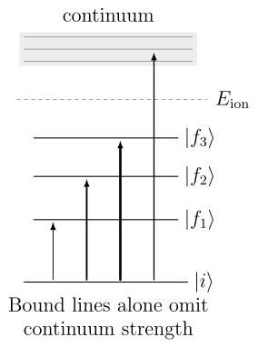
Bound lines and ionization channels share the total oscillator strength. This schematic shows upward transitions from a ground state; arrow widths indicate relative strengths only. For an excited initial state, downward transitions also enter the sum with negative signs.

Atomic Notation

Fine-structure lines

For a line

$$\gamma_iJ_i \longrightarrow \gamma_fJ_f,$$

the standard level weights are

$$g_i=2J_i+1, \qquad g_f=2J_f+1.$$

Atomic line lists commonly use lower index $i$ and upper index $k$, writing $f_{ik}$ and $A_{ki}$. This is the same direction convention as $f_{if}$ and $A_{fi}$ used here.

Database column	Read as	Do not read as
$A_{ki}$	upper-to-lower emission rate for one listed channel	total inverse lifetime unless every lower channel is included
$g_kA_{ki}$	upper-weighted transition probability	absorption $gf$
$f_{ik}$	lower-to-upper absorption oscillator strength	probability of absorption during an experiment
$\log(gf)$	$\log_{10}(g_if_{ik})$	$\log_{10}f_{ik}$
$S$ for E1	reduced dipole matrix element squared	oscillator strength without energy and degeneracy factors
relative intensity	source- and population-dependent line signal	intrinsic transition probability

The NIST Atomic Spectra Database also supplies accuracy codes and references to the original calculations or measurements. A converted value inherits the source uncertainty; conversion does not turn a theoretical or semiempirical entry into a direct measurement.

Terms and multiplets

For an unresolved LS term, a term weight may be defined by

$$g_{\mathrm{term}} = \sum_J(2J+1) = (2S+1)(2L+1).$$

A multiplet line strength is a sum over its component line strengths:

$$S_{\mathrm M} = \sum_{\mathrm{lines}}S_{\mathrm{line}}.$$

An unweighted sum of component oscillator strengths is generally not the term-averaged multiplet oscillator strength because each component has its own lower-level weight and transition energy. Convert components to a common weighted convention before summing.

Hyperfine-resolved data

For a hyperfine level with total angular momentum $F$,

$$g_F=2F+1.$$

Use this weight only when the reported strength is genuinely resolved and averaged at the hyperfine-level scale. A fine-structure oscillator strength does not acquire a new $g_F$ merely because a later calculation partitions it among hyperfine components. With no mixing between electronic $J$ levels, summing final hyperfine components and averaging initial ones with weights $(2F_i+1)/[(2I+1)(2J_i+1)]$ reconstructs the electronic strength when hyperfine frequency differences are neglected. The corresponding dipole-strength sum is exact in that angular model; oscillator strengths carry each component’s actual transition energy. A prepared single $F_i$ or $M_i$ is a different initial ensemble.

Molecular Notation

Molecular tables use “oscillator strength” for several nested objects. Always attach explicit quantum labels.

Molecular object	Example notation	Matrix element or sum represented
fixed-geometry electronic transition	$f_{if}(Q)$	electronic transition moment at nuclear geometry $Q$
vibronic line or band origin	$f_{v'v''}$	nuclear-motion integral of the coordinate-dependent electronic moment
rotational line	$f_{J'J''}$	one branch component with rotational angular factors
unresolved band	$f_{\mathrm{band}}$	declared sum over vibronic and/or rotational components
continuum strength	$df/dE$	density whose integral gives a dimensionless strength

Electronic and vibronic moments

For nuclear coordinates $Q$, an electronic transition moment is

$$\boldsymbol{\mu}_{fi}(Q) = \left\langle \psi_f(\mathbf r;Q) \left| \widehat{\mathbf D} \right| \psi_i(\mathbf r;Q) \right\rangle_{\mathbf r}.$$

The vibronic transition moment is

$$\mathbf D_{v'v''} = \int dQ\, \chi_{v'}^*(Q) \boldsymbol{\mu}_{fi}(Q) \chi_{v''}(Q).$$

In the Condon approximation, $\boldsymbol{\mu}_{fi}(Q)$ is replaced by a nearly constant value. The Franck–Condon factor then distributes squared overlap, but an oscillator strength still includes the individual transition energy:

$$f_{v'v''} \propto \Delta E_{v'v''} \left| \mathbf D_{v'v''} \right|^2.$$

Consequently, Franck–Condon fractions and oscillator-strength fractions are not exactly identical when the line energies differ. Coordinate dependence of the electronic moment introduces Herzberg–Teller intensity.

Rotational branches

Rotational line strengths are often written schematically as

$$S_{J'J''} = H_{J'J''} S_{\mathrm{vibronic}},$$

where $H_{J'J''}$ is a Hönl–London factor in a stated normalization. Some tables normalize the branch factors to one; others normalize their sum to a degeneracy. Convert the rotational factors and lower-state populations separately. A thermal absorption spectrum is not obtained by summing intrinsic $f_{J'J''}$ values without populations.

Continuum normalization

A continuum state normalized per unit energy gives a differential strength $df/dE$. One normalized per unit momentum or frequency gives a different density:

$$\frac{df}{dE}\,dE = \frac{df}{dk}\,dk = \frac{df}{d\omega}\,d\omega.$$

Only the integrated strength over the same physical interval is invariant. Quoting a continuum “oscillator strength” without its density variable and units is incomplete.

Comparing approximate calculations

For a local nonrelativistic electronic Hamiltonian,

$$\mathbf P=\frac{im_e}{\hbar}[H,\mathbf R], \qquad \mathbf R=\sum_a\mathbf r_a,\quad \mathbf P=\sum_a\mathbf p_a.$$

Exact eigenstates therefore give the same oscillator strength in length and velocity forms. A nonlocal effective potential contributes to the commutator; simply replacing the velocity operator by $\mathbf P/m_e$ can then be wrong even for converged eigenstates.

For compatible operators and nonzero strengths, the symmetric difference

$$\delta_{\rm LV}= \frac{|f^{(\rm L)}-f^{(\rm V)}|} {\tfrac12(|f^{(\rm L)}|+|f^{(\rm V)}|)}$$

can reveal approximation sensitivity. It is not a calibrated uncertainty: both forms can share the same model error. Weak transitions are especially sensitive to cancellations. Compare basis and correlation convergence as well as critically evaluated measurements (Kramida 2024).

Common pitfalls

An oscillator strength is not an absorption probability. It has no illumination time, photon flux, or line profile and need not lie below one. Use a cross section or transition-rate model to calculate a probability.

A bright emission line need not have a large intrinsic strength. For an optically thin source the total line power is proportional to $N_fA_{fi}h\nu_{fi}$, so the upper population matters. Collisions, cascades, self-absorption, and the detector can also alter the signal.

Magnetic-dipole and electric-quadrupole strengths use other conversions. Their operators, units, and frequency powers differ. Check the multipole before applying an E1 formula, even if a table labels the column simply “strength.”

Exercises

Reduced line strength and log(gf)

An atomic transition has $J_i=1$, $\Delta E=0.0750\,E_{\mathrm h}$, and $S_{if}=6.00\,e^2a_0^2$. Find $f_{if}$, $gf$, and $\log(gf)$.

Solution

The lower weight is

$$g_i=2J_i+1=3.$$

Therefore

$$\begin{aligned} f_{if} &= \frac{2}{3} \frac{0.0750}{3} (6.00) = 0.100, \\ gf &= 3(0.100) = 0.300, \\ \log(gf) &= \log_{10}(0.300) = -0.5229. \end{aligned}$$

Taking $\log_{10}f$ instead would give $-1$, which is not the tabulated $\log(gf)$.

Convert a database A value

A listed E1 line has $\lambda=5000.0\,\mathring{\mathrm A}$, $A_{fi}=1.60\times10^7\,\mathrm{s^{-1}}$, $g_i=3$, and $g_f=5$. Find $f_{if}$ and $\log(gf)$.

Solution

Use the ångström form:

$$\begin{aligned} f_{if} &= 1.49919\times10^{-16} \frac{5}{3} (5000.0)^2 (1.60\times10^7) \\ &= 0.09995. \end{aligned}$$

Then

$$\begin{aligned} gf &= 3(0.09995) = 0.2998, \\ \log(gf) &= \log_{10}(0.2998) = -0.5231. \end{aligned}$$

Had the numerical value $1.60\times10^7$ been interpreted as a column in units of $10^8\,\mathrm{s^{-1}}$, the result would be inconsistent with the printed entry.

Complete an excited-state sum

For a two-electron system in an excited state, the known upward oscillator strengths sum to $1.35$. The signed downward contributions sum to $-0.20$. How much bound-plus-continuum strength remains unaccounted for?

Solution

The target is $N=2$. The known signed sum is

$$F_{\mathrm{known}} = 1.35-0.20 = 1.15.$$

Therefore

$$F_{\mathrm{missing}} = 2.00-1.15 = 0.85.$$

Adding the downward magnitude as $+0.20$ would incorrectly reduce the missing strength to $0.45$.

Change the absorption axis

A line has $f_{if}=0.125$. Find its integrated cross section on an ordinary-frequency axis and on an angular-frequency axis.

Solution

On the ordinary-frequency axis,

$$\begin{aligned} \int\sigma_\nu\,d\nu &= (2.6540\times10^{-6})(0.125) \\ &= 3.3175\times10^{-7} \ \mathrm{m^2\,Hz}. \end{aligned}$$

The angular-frequency area is larger by $2\pi$:

$$\begin{aligned} \int\sigma_\omega\,d\omega &= 2\pi \int\sigma_\nu\,d\nu \\ &= 2.0845\times10^{-6} \ \mathrm{m^2\,rad\,s^{-1}}. \end{aligned}$$

The cross section at each photon energy is unchanged; its normalized profile and integration coordinate have changed.

Vibronic partition with unequal energies

In the Condon approximation, two vibronic channels have Franck–Condon factors $q_1=0.70$ and $q_2=0.30$. Their transition energies are $0.080\,E_{\mathrm h}$ and $0.100\,E_{\mathrm h}$, respectively. Neglect all other differences. What fractions of the two-channel oscillator strength do they carry?

Solution

Oscillator strength scales as $\Delta E q$ in this approximation:

$$w_1 = (0.080)(0.70) = 0.056,$$ $$w_2 = (0.100)(0.30) = 0.030.$$

After normalization,

$$\begin{aligned} \eta_1 &= \frac{0.056}{0.086} = 0.651, \\ \eta_2 &= \frac{0.030}{0.086} = 0.349. \end{aligned}$$

The Franck–Condon distribution is $70{:}30$, but the oscillator-strength distribution is approximately $65.1{:}34.9$ because the transition energies differ.

References

• Hilborn, Robert C. “Einstein coefficients, cross sections, $f$ values, dipole moments, and all that.” American Journal of Physics 50, 982–986 (1982). doi:10.1119/1.12937. Revised author version (2002).
• Kramida, Alexander. “Evaluation of uncertainties in atomic data on spectral lines and transition probabilities.” European Physical Journal D 78, 36 (2024). doi:10.1140/epjd/s10053-024-00820-y; NIST author copy.
• Kramida, Alexander, Yuri Ralchenko, Joseph Reader, and NIST ASD Team. NIST Atomic Spectra Database, Standard Reference Database 78. Database; doi:10.18434/T4W30F. Accessed 2026-10-14.
• Martin, William C., Wolfgang L. Wiese, and Alexander Kramida. “Spectral Lines: Selection Rules, Intensities, Transition Probabilities, Values, and Line Strengths”, in Atomic Spectroscopy: An Introduction. NIST, accessed 2026-10-14.
• Sobelman, Igor I. Atomic Spectra and Radiative Transitions, 2nd ed. Springer (1992). doi:10.1007/978-3-642-76907-8. Derivations and angular-momentum conventions underlying the atomic formulas.