Einstein Coefficient Reference

Einstein coefficients describe absorption, stimulated emission, and spontaneous emission between two declared levels in a weak-field rate model. For a lower level $1$, an upper level $2$, and a narrow transition at $\omega_0=(E_2-E_1)/\hbar>0$,

$$\begin{aligned} R_{1\rightarrow2}^{(\mathrm{abs})} &= B_{12}^{(\omega)} u_\omega(\omega_0), \\ R_{2\rightarrow1}^{(\mathrm{down})} &= A_{21} + B_{21}^{(\omega)} u_\omega(\omega_0). \end{aligned}$$

Here $u_\omega$ is the total isotropic radiation energy density per unit angular frequency. The superscript on $B$ is essential: a $B$ coefficient has a numerical value only relative to the spectral density, directional average, polarization sum, and line-profile convention that it multiplies.

The same transition can have different numerical $B$ coefficients when radiation is expressed per hertz or per radian per second. The observable transition rate must be unchanged. This reference explains those conversions and connects channel rates to lifetimes, branching fractions, and photon yields.

Helpful background. Einstein Coefficients derives the relations from thermal equilibrium and explains the three radiative processes.

Levels, radiation, and rates

Unless a section says otherwise:

• $E_2>E_1$ and $\omega_0=(E_2-E_1)/\hbar$;
• $g_1$ and $g_2$ are the total degeneracies of the lower and upper objects;
• populations are uniform within each degenerate level;
• $A_{21}$ describes one declared upper-to-lower radiative channel;
• $u_\omega(\omega)$ is total isotropic radiation energy in free space per volume per angular-frequency interval, summed over directions and both transverse polarizations;
• line profiles are normalized to unit area in the variable printed in their subscript;
• the narrow-line approximation is used only when the radiation density is nearly constant across the profile; and
• microscopic matrix-element formulas refer to an electric-dipole, or E1, transition in free space.

Here $u_\omega$ counts energy in occupied photon modes; it excludes the zero-point term $\hbar\omega/2$ per mode. Spontaneous emission is already included through $A$, so adding vacuum energy to $u_\omega$ would count part of the vacuum contribution twice.

The three coefficients are intrinsic to the declared transition model. A rate additionally requires a radiation field or a prepared upper-state population.

Core Definitions

Quantity	Definition	SI units
$A_{21}$	spontaneous rate per excited system	$\mathrm{s^{-1}}$
$B_{12}^{(\omega)}$	absorption rate divided by $u_\omega$	$\mathrm{m^3\,J^{-1}\,s^{-2}}$
$B_{21}^{(\omega)}$	stimulated-emission rate divided by $u_\omega$	$\mathrm{m^3\,J^{-1}\,s^{-2}}$
$g_2A_{21}$	upper-weighted rate	$\mathrm{s^{-1}}$
$\sum_\ell A_{2\ell}$	inverse radiative lifetime	$\mathrm{s^{-1}}$

Spontaneous coefficient

The coefficient $A_{21}$ is a conditional rate: if the atom is still in level $2$ at time $t$, the probability of a spontaneous transition to level $1$ during a short interval $dt$ is

$$\Pr(2\to1\text{ in }[t,t+dt]\mid 2\text{ at }t)=A_{21}\,dt+o(dt).$$

For an initially excited atom with no repumping and total first-order loss rate $\Gamma_{\rm tot}$, the surviving upper population is $p_2(t)=e^{-\Gamma_{\rm tot}t}$. The cumulative probability of decay through this channel is

$$P_{21}(t)=\frac{A_{21}}{\Gamma_{\rm tot}} (1-e^{-\Gamma_{\rm tot}t}), \qquad \frac{dP_{21}}{dt}=A_{21}p_2(t).$$

Thus $dP_{21}/dt$ decreases as the initial population is depleted, even when $A_{21}$ is constant.

For $N_2(t)$ independent emitters currently in the upper level, and before collection or detector losses,

$$\dot N_{\gamma,21} = N_2A_{21},$$

and the emitted optical power in that channel is

$$\mathcal P_{21} = N_2\hbar\omega_0A_{21}.$$

Atomic databases often call $A_{21}$ a transition probability. Its units show that it is a probability rate, not a dimensionless finite-time probability.

Stimulated coefficients

The absorption and stimulated-emission rates per system are

$$R_{1\rightarrow2}^{(\mathrm{abs})} = B_{12}^{(\omega)}u_\omega(\omega_0),$$ $$R_{2\rightarrow1}^{(\mathrm{stim})} = B_{21}^{(\omega)}u_\omega(\omega_0).$$

With

$$[u_\omega] = \mathrm{J\,m^{-3}} \left(\mathrm{rad\,s^{-1}}\right)^{-1},$$

and radians treated as dimensionless,

$$[B^{(\omega)}] = \mathrm{m^3\,J^{-1}\,s^{-2}}.$$

A $B$ coefficient alone is not a rate. It becomes one only after multiplication by the matching spectral energy density.

Finite Profiles

Let the absorption profile be normalized by

$$\int_0^\infty \phi_{12}^{(\omega)}(\omega)\,d\omega = 1.$$

The weak-field rate is

$$R_{1\rightarrow2}^{(\mathrm{abs})} = B_{12}^{(\omega)} \int_0^\infty u_\omega(\omega) \phi_{12}^{(\omega)}(\omega)\,d\omega.$$

Only when $u_\omega$ changes negligibly across the line may one write

$$R_{1\rightarrow2}^{(\mathrm{abs})} \simeq B_{12}^{(\omega)}u_\omega(\omega_0).$$

The spontaneous coefficient may likewise be distributed over a normalized emission profile:

$$\frac{dA_{21}}{d\omega} = A_{21}\phi_{21}^{(\omega)}(\omega), \qquad \int_0^\infty \frac{dA_{21}}{d\omega}\,d\omega = A_{21}.$$

The integrated $A$ and the line profile are separate objects. Broad vibronic bands, overlapping transitions, or rapidly varying radiation fields require the integral rather than a line-center shortcut.

Spectral-Density Conventions

Spectral energy is invariant under a coordinate change:

$$u_x(x)\,|dx| = u_y(y)\,|dy|.$$

For the narrow-line expression, the numerical $B$ changes inversely to the density so that the physical rate remains invariant:

$$B^{(x)}u_x = B^{(y)}u_y.$$

Angular frequency and ordinary frequency

Because

$$\omega=2\pi\nu, \qquad u_\nu(\nu)=2\pi u_\omega(\omega),$$

the coefficients satisfy

$$B_{ij}^{(\nu)} = \frac{1}{2\pi} B_{ij}^{(\omega)}.$$

The two conventions have the same reduced SI dimensions when radians are dimensionless, so dimensional analysis does not reveal a missing $2\pi$.

Spectroscopic wavenumber

For $\widetilde\nu=\nu/c$ measured in $\mathrm{m^{-1}}$,

$$u_{\widetilde\nu} = c\,u_\nu, \qquad B_{ij}^{(\widetilde\nu)} = \frac{1}{c} B_{ij}^{(\nu)}.$$

If wavenumber is measured in $\mathrm{cm^{-1}}$, then

$$B_{ij}^{(\mathrm{cm}^{-1})} = \frac{1}{100c} B_{ij}^{(\nu)}.$$

The unit attached to the wavenumber variable is part of the coefficient definition.

Wavelength

Since $\nu=c/\lambda$,

$$u_\lambda(\lambda) = \frac{c}{\lambda^2} u_\nu(\nu).$$

At a narrow line centered on $\lambda_0$,

$$B_{ij}^{(\lambda)} = \frac{\lambda_0^2}{c} B_{ij}^{(\nu)}.$$

For a finite profile, transform the whole rate integral. With a normalized frequency profile $\phi_\nu$,

$$\begin{aligned} R&=B^{(\nu)}\int u_\nu(\nu)\phi_\nu(\nu)\,d\nu\\ &=\int u_\lambda(\lambda)\, B^{(\nu)}\phi_\nu(c/\lambda)\,d\lambda. \end{aligned}$$

If one uses the normalized wavelength profile $\phi_\lambda(\lambda)=\phi_\nu(c/\lambda)c/\lambda^2$ instead, the coefficient inside the integral must be $B^{(\lambda)}(\lambda)=B^{(\nu)}\lambda^2/c$. Replacing it by the value at $\lambda_0$ requires a narrow line. This is why independently transforming both the radiation density and the profile while leaving $B$ unchanged gives the wrong rate.

Conversion table

Density used in the rate	Coordinate units	Coefficient relative to $B^{(\omega)}$
$u_\omega$	$\mathrm{rad\,s^{-1}}$	$B^{(\omega)}$
$u_\nu$	$\mathrm{Hz}$	$B^{(\nu)}=B^{(\omega)}/(2\pi)$
$u_{\widetilde\nu}$	$\mathrm{m^{-1}}$	$B^{(\widetilde\nu)}=B^{(\omega)}/(2\pi c)$
$u_{\widetilde\nu}$	$\mathrm{cm^{-1}}$	$B^{(\mathrm{cm}^{-1})}=B^{(\omega)}/(200\pi c)$
$u_\lambda$ near $\lambda_0$	$\mathrm m$	$B^{(\lambda)}=\lambda_0^2B^{(\omega)}/(2\pi c)$

Relations Among the Coefficients

For sharp levels in free space and the conventions above, thermal detailed balance gives (Hilborn 2002)

$$g_1B_{12}^{(\omega)} = g_2B_{21}^{(\omega)}.$$

Thus

$$B_{12}^{(\omega)} = \frac{g_2}{g_1} B_{21}^{(\omega)}.$$

The two level-averaged $B$ coefficients are equal only when the degeneracies are equal. For matched resolved substates, isotropic absorption and stimulated-emission coefficients are equal by Hermiticity of the dipole operator. Summing over final substates and averaging over initial ones introduces the different degeneracy factors. See the explicit Wigner–Eckart convention in the oscillator-strength reference.

The spontaneous-to-stimulated relation is

$$\frac{A_{21}} {B_{21}^{(\omega)}} = \frac{\hbar\omega_0^3} {\pi^2c^3}.$$

In ordinary-frequency notation,

$$\frac{A_{21}} {B_{21}^{(\nu)}} = \frac{8\pi h\nu_0^3} {c^3}.$$

These are the same physical relation expressed with different spectral densities. Thermodynamic balance fixes ratios among coefficients; it does not determine their absolute scale. The transition matrix element supplies that scale.

Thermal Radiation Lookup

The mean occupation of a thermal photon mode is

$$\overline n(\omega_0,T) = \frac{1} { \exp\!\left( \dfrac{\hbar\omega_0}{k_{\mathrm B}T} \right)-1 }.$$

Planck’s energy density per angular frequency is

$$u_\omega(\omega_0,T) = \frac{\hbar\omega_0^3} {\pi^2c^3} \overline n.$$

Using the Einstein relations gives the compact rates

$$R_{2\rightarrow1}^{(\mathrm{th})} = A_{21}(\overline n+1),$$ $$R_{1\rightarrow2}^{(\mathrm{th})} = \frac{g_2}{g_1} A_{21}\overline n.$$

The $+1$ is the spontaneous contribution. The thermal population ratio

$$\frac{N_2}{N_1} = \frac{g_2}{g_1} \exp\!\left( -\frac{\hbar\omega_0}{k_{\mathrm B}T} \right)$$

ensures

$$N_1R_{1\rightarrow2}^{(\mathrm{th})} = N_2R_{2\rightarrow1}^{(\mathrm{th})}.$$

For optical transitions at room temperature, $\overline n$ is usually negligible. For microwave and radio-frequency transitions it can be much larger than one.

Lifetimes and Branching

Total radiative width

If level $2$ has several radiative channels,

$$\Gamma_{\mathrm{rad},2} = \sum_\ell A_{2\ell}.$$

The radiative lifetime is

$$\tau_{\mathrm{rad},2} = \frac{1} {\Gamma_{\mathrm{rad},2}}.$$

One channel coefficient equals the inverse radiative lifetime only when it is the sole radiative decay channel.

Branching fractions

The radiative branching fraction into channel $2\rightarrow\ell$ is

$$b_{2\ell}^{(\mathrm{rad})} = \frac{A_{2\ell}} {\sum_jA_{2j}}, \qquad \sum_\ell b_{2\ell}^{(\mathrm{rad})} = 1.$$

Conversely, if a radiative lifetime and complete radiative branching fractions are known,

$$A_{2\ell} = \frac{ b_{2\ell}^{(\mathrm{rad})} }{ \tau_{\mathrm{rad},2} }.$$

Observed lifetime and quantum yield

With additional first-order channels,

$$\Gamma_{\mathrm{tot},2} = \Gamma_{\mathrm{rad},2} + \Gamma_{\mathrm{nr},2} + \Gamma_{\mathrm{coll},2} + \cdots,$$

and

$$\tau_{\mathrm{obs},2} = \frac{1} {\Gamma_{\mathrm{tot},2}}.$$

The radiative quantum yield is

$$\Phi_{\mathrm{rad}} = \frac{\Gamma_{\mathrm{rad},2}} {\Gamma_{\mathrm{tot},2}} = \frac{\tau_{\mathrm{obs},2}} {\tau_{\mathrm{rad},2}}.$$

These expressions assume no repumping, no population feeding from other levels, and no double counting of loss channels: for example, if $\Gamma_{\rm nr}$ already includes collisional quenching, do not add it again as $\Gamma_{\rm coll}$. The probability that one initially excited atom emits on a particular branch is

$$\Phi_{2\ell}=\frac{A_{2\ell}}{\Gamma_{\rm tot,2}} =\Phi_{\rm rad}\,b_{2\ell}^{(\rm rad)}.$$

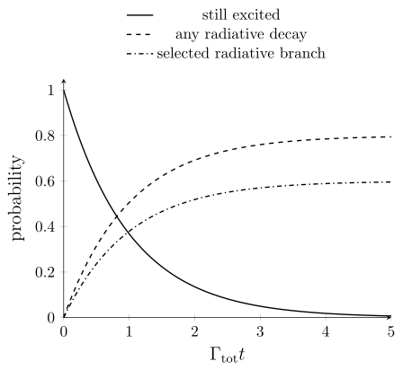
For the rates in the first exercise, the atom has an $80\%$ probability of emitting any photon and a $60\%$ probability of emitting on the selected branch. The surviving population falls exponentially. A constant channel rate $A_{21}$ does not mean a constant probability per unit time for the original ensemble.

The lifetime ratio assumes the same state and first-order kinetics. In multiexponential, transfer-coupled, diffusion-limited, or time-dependent environments, no single reciprocal rate need describe the measured trace.

Natural Width

For a stable lower state, only spontaneous radiative upper-state loss, no pure dephasing, and exponential decay,

$$\Gamma_1 = \sum_\ell A_{2\ell}, \qquad \Gamma_2 = \frac{\Gamma_1}{2}.$$

The Lorentzian full width at half maximum is then

$$\Delta\omega_{\mathrm{FWHM}} = \Gamma_1,$$

or

$$\Delta\nu_{\mathrm{FWHM}} = \frac{\Gamma_1}{2\pi}.$$

For independent Markovian loss channels and an isolated optical coherence, more generally,

$$\Gamma_2 = \frac{\Gamma_{\mathrm{upper}} +\Gamma_{\mathrm{lower}}}{2} + \gamma_\phi,$$

so

$$\Delta\omega_{\mathrm{FWHM}} = 2\Gamma_2.$$

The radiative natural width uses the sum of the relevant spontaneous $A$ channels, including radiative loss from the lower level if applicable. Nonradiative loss and pure dephasing contribute to the broader homogeneous linewidth; they are not additional Einstein $A$ coefficients. Coherence transfer or correlated reservoirs can require coupled equations. See the Line Shape Reference.

Electric-Dipole Conversions

Nondegenerate transition dipole

For

$$\mathbf d_{21} = \langle2| \widehat{\mathbf D} |1\rangle,$$

the free-space E1 coefficients are

$$A_{21} = \frac{\omega_0^3} {3\pi\epsilon_0\hbar c^3} \left|\mathbf d_{21}\right|^2,$$ $$B_{21}^{(\omega)} = \frac{\pi} {3\epsilon_0\hbar^2} \left|\mathbf d_{21}\right|^2.$$

For nondegenerate endpoints,

$$B_{12}^{(\omega)} = B_{21}^{(\omega)}.$$

Degenerate levels and reduced line strength

For a reduced E1 line strength

$$S_{21} = \left| \left\langle \gamma_2J_2 \left\| \widehat D^{(1)} \right\| \gamma_1J_1 \right\rangle \right|^2,$$

the level-averaged coefficients are

$$\begin{aligned} A_{21} &= \frac{\omega_0^3} {3\pi\epsilon_0\hbar c^3g_2} S_{21}, \\ B_{21}^{(\omega)} &= \frac{\pi} {3\epsilon_0\hbar^2g_2} S_{21}, \\ B_{12}^{(\omega)} &= \frac{\pi} {3\epsilon_0\hbar^2g_1} S_{21}. \end{aligned}$$

The spontaneous and stimulated-emission coefficients average over upper substates; the absorption coefficient averages over lower substates.

Relation to oscillator strength

For an E1 absorption oscillator strength $f_{12}$,

$$A_{21} = \frac{e^2\omega_0^2} {2\pi\epsilon_0m_ec^3} \frac{g_1}{g_2} f_{12}.$$

The angular-frequency stimulated coefficients are

$$B_{12}^{(\omega)} = \frac{\pi e^2} {2\epsilon_0m_e\hbar\omega_0} f_{12},$$ $$B_{21}^{(\omega)} = \frac{g_1}{g_2} B_{12}^{(\omega)}.$$

For vacuum wavelength in ångströms and $A_{21}$ in $\mathrm{s^{-1}}$,

$$f_{12} = 1.49919\times10^{-16} \frac{g_2}{g_1} \lambda_{\mathring{\mathrm A}}^{\,2} A_{21}.$$

For $S_{21}$ in $e^2a_0^2$,

$$A_{21} = \frac{2.02613\times10^{18}} {g_2\lambda_{\mathring{\mathrm A}}^{\,3}} S_{21}.$$

Conversions among $f$, $gf$, $\log(gf)$, and $S$ are collected in Oscillator Strength Reference.

Fixed-strength frequency scaling

For a fixed E1 line strength,

$$A_{21}\propto\omega_0^3, \qquad B_{21}^{(\omega)} \propto S_{21}.$$

For a fixed oscillator strength, however,

$$A_{21}\propto\omega_0^2, \qquad B_{12}^{(\omega)} \propto\omega_0^{-1}.$$

Always state which structural quantity is being held fixed before quoting a frequency scaling.

Beyond Free-Space E1

Einstein $A$ values are also used for M1, E2, and higher-multipole transitions. Their microscopic operators, dimensions, angular factors, and frequency powers differ from the E1 formulas above. The transition type must be read before converting a database line strength.

In a cavity, waveguide, dielectric, photonic crystal, near a surface, or in another structured reservoir, spontaneous emission depends on the local electromagnetic density of states and mode functions. A vacuum $A$ can be enhanced, suppressed, redirected, or split among channels. Use a mode-resolved calculation or electromagnetic Green tensor rather than silently applying the free-space formula.

The equilibrium relations among upward and downward processes also assume a specified reservoir and consistent mode normalization. They are not a universal recipe for replacing an environment-dependent decay rate while leaving every other coefficient unchanged.

Atomic Database Notation

Atomic line lists commonly use lower level $i$ and upper level $k$:

$$i\rightarrow k \quad\text{for absorption}, \qquad k\rightarrow i \quad\text{for emission}.$$

Column	Meaning	Required check
$A_{ki}$	spontaneous upper-to-lower rate	$\mathrm{s^{-1}}$ or units of $10^8\,\mathrm{s^{-1}}$
$g_kA_{ki}$	upper-weighted rate	use $g_k=2J_k+1$ for a fine-structure level
accuracy code	assessed uncertainty category	retain the cited transition-probability reference
type	E1, M1, E2, mixed, induced, or other	choose the matching line-strength formula
relative intensity	source-dependent observed strength	do not equate with $A_{ki}$

The lifetime of upper level $k$ requires all radiative channels:

$$\tau_{\mathrm{rad},k}^{-1} = \sum_i A_{ki}.$$

A search window, wavelength table, or detector band may omit important branches. Sum over the level’s complete transition set, not merely the lines visible in one query.

Molecular Database Notation

Molecular $A_{ji}$ values refer to fully or partially resolved rovibronic transitions. Statistical weights can include rotational, electronic, nuclear-spin, parity, and symmetry factors. The same convention must be used in the line list and its partition function.

HITRAN, for example, stores a temperature-independent $A_{ji}$ in $\mathrm{s^{-1}}$, while its line intensity is temperature dependent. In HITRAN’s wavenumber and cgs-style convention,

$$S_{ij}^{(\mathrm{HIT})}(T) = I_{\mathrm a} \frac{A_{ji}} {8\pi c\widetilde\nu_{ij}^{\,2}} \frac{ g_j \exp(-c_2E_i/T) }{ Q(T) } \times \left[ 1-\exp(-c_2\widetilde\nu_{ij}/T) \right],$$

where:

• $S_{ij}^{(\mathrm{HIT})}$ has units $\mathrm{cm^{-1}/(molecule\,cm^{-2})}$, equivalently $\mathrm{cm\,molecule^{-1}}$;
• $\widetilde\nu_{ij}$ and $E_i$ are in $\mathrm{cm^{-1}}$;
• $c$ is in $\mathrm{cm\,s^{-1}}$;
• $c_2=hc/k_{\mathrm B}$ is in $\mathrm{cm\,K}$;
• $g_j$ is the upper-state statistical weight;
• $Q(T)$ uses the matching weight convention; and
• $I_{\mathrm a}$ is the terrestrial isotopologue abundance factor used by the database.

The database line intensity $S_{ij}^{(\mathrm{HIT})}$ is not the reduced matrix-element line strength $S_{21}$ used in the E1 formulas. The shared letter $S$ does not make them the same physical quantity.

When population equations suffice

Einstein coefficients describe incoherent absorption and emission when the relevant rates are linear in the specified radiation density, the reservoir has short memory, and the assumed sublevel populations apply. Line overlap or coherently interfering pathways may require a response matrix rather than separate scalar profiles.

Population saturation is possible in a rate equation. For an isolated pair of levels, the incoherent equation

$$\dot N_2=N_1B_{12}u-N_2(A_{21}+B_{21}u)$$

gives $N_2/N_1\to g_2/g_1$ as the stimulated rates become much larger than $A_{21}$, as long as the rate approximation remains valid. The populations saturate even though each induced rate remains linear in $u$. This limit gives equal populations per magnetic substate, not equal total level populations when $g_1\ne g_2$.

Coherent driving asks for more information. A laser can create optical coherences, Rabi oscillations, dark states, and power broadening. Use Optical Bloch Equations when these matter. A collimated irradiance is not the isotropic spectral energy density used above; field amplitude, polarization, and the transition dipole determine its coupling.

A constant spontaneous rate requires an appropriate reservoir. Strong coupling, memory effects, or a structured electromagnetic environment can invalidate exponential decay. The relevant starting points are Spontaneous Emission and the Quantum Optical Master Equation.

Exercises

Lifetime, branching, and quantum yield

An upper level has radiative channels $A_{21}=3.0\times10^7\,\mathrm{s^{-1}}$ and $A_{20}=1.0\times10^7\,\mathrm{s^{-1}}$, plus a nonradiative rate $\Gamma_{\mathrm{nr}}=1.0\times10^7\,\mathrm{s^{-1}}$. Find the radiative lifetime, radiative branching fraction into level $1$, observed lifetime, and radiative quantum yield.

Solution

The radiative rate is

$$\Gamma_{\mathrm{rad}} = 3.0\times10^7+1.0\times10^7 = 4.0\times10^7\ \mathrm{s^{-1}}.$$

Therefore

$$\tau_{\mathrm{rad}} = \frac{1}{4.0\times10^7} = 25\ \mathrm{ns}.$$

The radiative branching fraction is

$$b_{21}^{(\mathrm{rad})} = \frac{3.0}{4.0} = 0.75.$$

Including the nonradiative channel,

$$\Gamma_{\mathrm{tot}} = 5.0\times10^7\ \mathrm{s^{-1}}, \qquad \tau_{\mathrm{obs}} = 20\ \mathrm{ns}.$$

Finally,

$$\Phi_{\mathrm{rad}} = \frac{4.0}{5.0} = 0.80.$$

The single channel $A_{21}$ is therefore not the inverse lifetime in this example.

Degeneracy and spectral convention

Suppose $g_1=2$, $g_2=6$, and $B_{21}^{(\omega)}=4.00\times10^{20}$ in the matching SI units. Find $B_{12}^{(\omega)}$ and $B_{12}^{(\nu)}$.

Solution

Detailed balance gives

$$B_{12}^{(\omega)} = \frac{g_2}{g_1} B_{21}^{(\omega)} = 3(4.00\times10^{20}) = 1.20\times10^{21}.$$

Changing from angular to ordinary frequency,

$$\begin{aligned} B_{12}^{(\nu)} &= \frac{B_{12}^{(\omega)}}{2\pi} \\ &= 1.91\times10^{20}. \end{aligned}$$

The degeneracy factor and the $2\pi$ Jacobian answer different questions and must both be applied.

Thermal detailed balance

For a transition with $A_{21}=1.00\times10^7\,\mathrm{s^{-1}}$, $g_2/g_1=3$, and thermal occupation $\overline n=0.20$, find the upward and downward rates per system. Verify event balance using the equilibrium population ratio.

Solution

The downward rate per upper-state system is

$$R_{2\rightarrow1} = A_{21}(\overline n+1) = 1.20\times10^7\ \mathrm{s^{-1}}.$$

The upward rate per lower-state system is

$$R_{1\rightarrow2} = \frac{g_2}{g_1} A_{21}\overline n = 6.00\times10^6\ \mathrm{s^{-1}}.$$

The Bose factor implies

$$e^{-\hbar\omega_0/(k_{\mathrm B}T)} = \frac{\overline n}{\overline n+1} = \frac{1}{6}.$$

Hence

$$\frac{N_2}{N_1} = 3\left(\frac{1}{6}\right) = \frac{1}{2}.$$

Therefore

$$N_1(6.00\times10^6) = N_2(1.20\times10^7),$$

as required.

Microwave thermal occupation

Estimate the thermal photon occupation at $\nu_0=10.0\,\mathrm{GHz}$ and $T=300\,\mathrm K$. Is spontaneous emission the dominant downward contribution?

Solution

The dimensionless ratio is

$$\frac{h\nu_0}{k_{\mathrm B}T} = 1.600\times10^{-3}.$$

Thus

$$\overline n = \frac{1} {\exp(1.600\times10^{-3})-1} = 624.6.$$

The stimulated downward contribution is $A_{21}\overline n$, whereas the spontaneous contribution is $A_{21}$. Thermal stimulated emission is therefore about $625$ times larger than the extra spontaneous term. Room-temperature microwave experiments must account for thermal photons.

Conditional rate and cumulative probability

Use the rates of the first exercise. What is the probability that an initially excited atom has emitted a photon on branch $2\to1$ after $20$ ns? What is the instantaneous rate of this event per originally excited atom at that time?

Solution

The total decay rate is $5.0\times10^7\ {\rm s^{-1}}$, so $\Gamma_{\rm tot}t=1$. Hence

$$P_{21}(t)=\frac{3}{5}(1-e^{-1})\simeq0.379,$$

while

$$\frac{dP_{21}}{dt}=A_{21}e^{-1} \simeq1.10\times10^7\ {\rm s^{-1}}.$$

The conditional rate for atoms that remain excited is still $A_{21}=3.0\times10^7\ {\rm s^{-1}}$.

References

• Hilborn, Robert C. “Einstein coefficients, cross sections, $f$ values, dipole moments, and all that.” American Journal of Physics 50, 982–986 (1982). doi:10.1119/1.12937. Revised author version (2002).
• HITRAN. “Definitions and Units”. Online documentation, accessed 2026-10-14. Source for the molecular line-intensity, statistical-weight, and isotopic-abundance conventions.
• Martin, William C., Wolfgang L. Wiese, and Alexander Kramida. “Spectral Lines: Selection Rules, Intensities, Transition Probabilities, Values, and Line Strengths”, in Atomic Spectroscopy: An Introduction. NIST, accessed 2026-10-14.
• Šimečková, M., D. Jacquemart, L. S. Rothman, R. R. Gamache, and A. Goldman. “Einstein $A$-coefficients and statistical weights for molecular absorption transitions in the HITRAN database.” Journal of Quantitative Spectroscopy and Radiative Transfer 98, 130–155 (2006). doi:10.1016/j.jqsrt.2005.07.003.
• Sobelman, Igor I. Atomic Spectra and Radiative Transitions, 2nd ed. Springer (1992). doi:10.1007/978-3-642-76907-8.