Laser Nomenclature

Laser terminology describes amplification in a material, energy stored in a resonator, and coherent driving of atoms. These processes use related quantities, but their definitions differ. For example, a cavity linewidth measures passive energy loss, while a laser output linewidth measures fluctuations of the oscillating field. This reference connects the gain, resonator, and two-level-atom conventions through their defining equations.

Helpful background. Lasers introduces gain, feedback, and output coupling. The derivations are developed in gain and threshold, optical cavities, and optical Bloch equations.

Gain

Power gain and field gain

For the amplified signal in a uniform active medium, define the net power-propagation equation

$$\frac{dI}{dz} = \left( g-\alpha \right)I.$$

After distance $L$,

$$\frac{I(L)}{I(0)} = \exp \left[ (g-\alpha)L \right].$$

The power gain is therefore

$$G_P = \frac{P_{\mathrm{out}}}{P_{\mathrm{in}}} = e^{(g-\alpha)L}$$

when input and output use the same transverse mode and wave impedance. This is the gain of the stimulated signal: spontaneous light added by the amplifier is a separate contribution to the total measured output.

If the complex field envelope obeys

$$\frac{d\mathcal E}{dz} = \frac12 \left( g-\alpha \right)\mathcal E,$$

then the field-amplitude magnitude is

$$\left| \frac{\mathcal E(L)}{\mathcal E(0)} \right| = e^{(g-\alpha)L/2}.$$

The factor of one half follows because power is proportional to field magnitude squared. A source may instead define $g$ as a field-amplitude coefficient. Its propagation equation, not the symbol, determines which meaning applies.

Local, integrated, and decibel gain

Name	Definition	Units
power-gain coefficient	$g(z)$	$\mathrm{m^{-1}}$
integrated gain exponent	$\int g(z)\,dz$	1
material power multiplier, excluding loss	$\exp(\int g\,dz)$	1
field gain	$G_E=\mathcal E_{\mathrm{out}}/\mathcal E_{\mathrm{in}}$	1
power gain in decibels	$10\log_{10}G_P$	dB
field-magnitude gain in decibels	$20\log_{10}\lvert G_E\rvert$	dB

The two decibel expressions agree when $G_P=\lvert G_E\rvert^2$. Decibels describe a ratio; “$3\,\mathrm{dB\,m^{-1}}$” is a logarithmic coefficient and must be converted before it is inserted into a natural exponential.

Material, modal, and net gain

The material gain is a local property of the active material under a declared pump, frequency, polarization, and population distribution. A resonator mode generally samples only part of that material. In a simple scalar approximation,

$$g_\mu = \Gamma_\mu g_{\mathrm{mat}},$$

where $\Gamma_\mu$ is a mode-overlap or confinement factor. The net modal gain is

$$g_{\mathrm{net},\mu} = g_\mu-\alpha_\mu.$$

In a nonuniform or vector problem, $\Gamma_\mu g_{\mathrm{mat}}$ is replaced by a field-weighted overlap integral. A quoted material gain does not establish that any cavity mode has positive net gain.

Small-signal and saturated gain

Small-signal gain is the linear response before the signal significantly changes the inversion or carrier distribution. A simple continuous-wave saturation model is

$$g(I) = \frac{g_0}{1+I/I_{g,\mathrm{sat}}},$$

where $g_0$ is small-signal gain and $I_{g,\mathrm{sat}}$ is a model-specific gain-saturation intensity.

This formula is not universal. Pulsed systems may be governed by a saturation fluence, and inhomogeneous gain, spectral hole burning, carrier transport, recovery dynamics, and standing-wave spatial hole burning require more structure. A gain value should therefore say whether it is small-signal, saturated, differential, or measured at a stated operating point.

Laser Threshold

Round-trip condition

Let the selected mode return after one cavity circuit with complex field multiplier $\lambda_\mu$. Its round-trip power multiplier is

$$\mathcal G_{\mathrm{rt},\mu} = \lvert\lambda_\mu\rvert^2.$$

The linear modal threshold is

$$\lvert\lambda_\mu\rvert=1,$$

or equivalently

$$\mathcal G_{\mathrm{rt},\mu}=1.$$

Below threshold the leading perturbation decays; above threshold it grows until nonlinear gain saturation and mode competition establish a new operating state. Positive single-pass gain is not enough: the mode must recover all distributed, mirror, diffraction, and output-coupling losses in one full circuit.

The phase condition also matters:

$$\arg\lambda_\mu = 2\pi q, \qquad q\in\mathbb Z.$$

The first lasing mode is a field distribution and frequency that satisfies both amplitude and phase self-consistency.

Uniform linear-cavity formula

For a linear cavity with one-way active length $L$, power reflectivities $R_1$ and $R_2$, modal overlap $\Gamma_m$, uniform material power gain $g_{\mathrm{mat}}$, and uniform distributed power loss $\alpha$,

$$\mathcal G_{\mathrm{rt}} = R_1R_2 \exp \left[ 2L \left( \Gamma_m g_{\mathrm{mat}}-\alpha \right) \right].$$

Threshold gives

$$g_{\mathrm{mat,th}} = \frac{1}{\Gamma_m} \left[ \alpha + \frac{1}{2L} \ln \left( \frac{1}{R_1R_2} \right) \right].$$

This expression uses power reflectivities and power-gain coefficients. A ring cavity counts each physical section according to the actual circuit; one must not import the linear cavity’s double pass automatically.

Which threshold?

Several experimentally quoted thresholds answer different questions:

Threshold label	Operational criterion
linear-stability threshold	leading round-trip eigenvalue reaches unit magnitude
pump threshold	external pump value corresponding to that modal condition
light–light kink	change in slope of output versus pump
coherence threshold	onset of a chosen first-order coherence signature
spectral threshold	emergence or narrowing of a selected oscillating line
high-$\beta$ crossover	smooth transition in a device with substantial spontaneous emission into the selected mode

In an ideal low-$\beta$ laser these criteria can nearly coincide. In high-$\beta$ nanolasers, multimode devices, or noisy systems they need not. State the observable used to locate threshold and the model used to infer gain-equals-loss.

Cavity Finesse and Quality Factor

Free spectral range and resonance width

The free spectral range is the separation between adjacent longitudinal resonances of the same mode family:

$$\nu_{\mathrm{FSR}} \simeq \frac{1}{t_{\mathrm{rt}}},$$

where $t_{\mathrm{rt}}$ is the round-trip group delay, including dispersive mirror phase when relevant. For a nondispersive linear cavity of physical length $L$ and refractive index $n$,

$$\nu_{\mathrm{FSR}} \simeq \frac{c}{2nL}.$$

For an isolated passive-cavity resonance, let $\Delta\nu_c$ be the power-response FWHM in hertz.

Finesse

The operational finesse is

$$\mathcal F = \frac{\nu_{\mathrm{FSR}}}{\Delta\nu_c}.$$

It compares a resonance width with the spacing to the next longitudinal resonance. Both numerator and denominator must use the same frequency coordinate and mode family.

The Airy coefficient is not the finesse. If $\rho$ is the round-trip field survival magnitude, an ideal Airy response can be written

$$\mathcal A_{\mathrm{cav}}(\phi) = \frac{1}{ 1+\mathscr F\sin^2(\phi/2) },$$

with

$$\mathscr F = \frac{4\rho}{(1-\rho)^2}.$$

For this ideal response, the half-maximum points obey $\sin^2(\phi/2)=1/\mathscr F$. Hence

$$\mathcal F=\frac{\pi}{2\arcsin[(1-\rho)/(2\sqrt\rho)]},$$

provided the response falls to half maximum between resonances. If $(1-\rho)/(2\sqrt\rho)>1$, it never does, so this FWHM is undefined. In the high-finesse limit,

$$\mathcal F \simeq \frac{\pi\sqrt{\rho}}{1-\rho}.$$

The calligraphic $\mathcal F$ and Airy $\mathscr F$ are deliberately different. At low finesse, with overlapping modes or background interference, fit the actual transfer function rather than relying on the high-finesse approximation.

Quality factor

For stored cavity energy $U$ and total loss power $P_{\mathrm{loss}}$,

$$Q = \omega_c \frac{U}{P_{\mathrm{loss}}}.$$

If the undriven energy decays as

$$U(t) = U(0)e^{-\kappa t},$$

then

$$P_{\mathrm{loss}} = \kappa U,$$

and

$$Q = \frac{\omega_c}{\kappa}.$$

Near an isolated Lorentzian resonance,

$$\Delta\omega_c=\kappa,$$

so

$$Q = \frac{\omega_c}{\Delta\omega_c} = \frac{\nu_c}{\Delta\nu_c}.$$

The photon or stored-energy lifetime is

$$\tau_p = \frac{1}{\kappa}.$$

Some sources define $\kappa$ as a field-amplitude decay rate: $\mathcal E\propto e^{-\kappa t}$. Under that convention, energy decays at $2\kappa$. Always translate from the stated time-domain law.

Finesse is not Q

For the isolated resonance and linewidth convention just stated,

$$Q = \frac{\nu_c}{\nu_{\mathrm{FSR}}} \mathcal F.$$

Finesse measures spectral isolation relative to adjacent cavity modes; $Q$ measures fractional resonance width relative to the optical carrier. The ratio $\nu_c/\nu_{\mathrm{FSR}}$ is approximately a longitudinal mode order. Two cavities can have the same $Q$ and different finesse.

The number of round-trip times contained in one stored-energy lifetime is approximately

$$\frac{\tau_p}{t_{\mathrm{rt}}} \simeq \frac{\mathcal F}{2\pi},$$

not $\mathcal F$. In a discrete round-trip model the exact energy decay constant is $\kappa=-2\ln\rho/t_{\rm rt}$. Its equality to the Airy power-response FWHM in angular frequency is a high-finesse approximation.

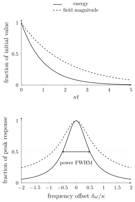
Solid curves show energy decay (top) and power response (bottom); dashed curves show field magnitude. An isolated damped cavity mode has field envelope $e^{-\kappa t/2}$ and energy $e^{-\kappa t}$. Its steady driven power response is $[1+(2\delta\omega/\kappa)^2]^{-1}$, with FWHM $\kappa$ in angular frequency. Taking the field magnitude instead of power changes both the decay time and the half-maximum width. These are passive-cavity properties.

Effective Mode Volume

Lossless nondispersive definition

For a well-confined mode of a lossless nondispersive dielectric cavity, an engineering mode volume referenced to the electric-energy-density maximum is

$$V_{\mathrm{cav}} = \frac{ \displaystyle \int \epsilon(\mathbf r) \lvert\mathbf E(\mathbf r)\rvert^2 d^3r }{ \displaystyle \max_{\mathbf r} \left[ \epsilon(\mathbf r) \lvert\mathbf E(\mathbf r)\rvert^2 \right] }.$$

The field normalization cancels. The quantity measures concentration of a particular mode, not the geometric volume enclosed by mirrors.

For an emitter at $\mathbf r_0$ with a real unit dipole direction (linear dipole), $\widehat{\mathbf e}_d$, a position- and orientation-dependent effective volume is

$$V_{\mathrm{eff}} \left( \mathbf r_0,\widehat{\mathbf e}_d \right) = \frac{ \displaystyle \int \epsilon(\mathbf r) \lvert\mathbf E(\mathbf r)\rvert^2 d^3r }{ \displaystyle \epsilon(\mathbf r_0) \left| \widehat{\mathbf e}_d \mathbin{\cdot} \mathbf E(\mathbf r_0) \right|^2 }.$$

An emitter at a node or with orthogonal polarization has a large or divergent effective volume even when the cavity’s maximum-referenced volume is small.

Gaussian standing-wave estimate

For a paraxial fundamental Gaussian standing wave in a homogeneous cavity, let $w_0$ be the $1/e$ field radius at a waist antinode and $L$ the cavity length. Neglect clipping and average over many standing-wave periods. Then

$$V_{\mathrm{cav}} \simeq \frac{\pi w_0^2L}{4}.$$

For an intensity envelope proportional to $(w_0/w(z))^2\exp[-2r^2/w(z)^2]$, the transverse integral is $\pi w_0^2/2$ at every $z$. Thus slow variation of the beam radius does not by itself spoil the estimate. Longitudinal standing-wave averaging supplies the other factor of one half. A traveling-wave mode with the same normalized envelope lacks that standing-wave factor. See optical cavities for the mode geometry.

Validity limits

The simple energy-density ratio is not universal. Open low-$Q$ resonators have leaky quasinormal modes; dispersive media change electromagnetic energy normalization; absorptive media can make a naive $\epsilon\lvert E\rvert^2$ integrand unsuitable; and degenerate modes require a basis choice. Those systems require generalized mode normalization; see Kristensen and Hughes (2014) and the cavity-QED discussion.

Small mode volume, high $Q$, and high finesse are independent design properties. A cavity can confine a mode tightly while losing energy rapidly, or store energy for a long time in a large spatial mode.

Linewidth and Coherence

Identify the object first

At least four widths occur in laser work:

Width	Object being measured	Typical cause
gain bandwidth	material amplification spectrum	transition distribution, collisions, carrier states
passive-cavity linewidth	driven cold-cavity power response	output coupling and internal loss
atomic or molecular linewidth	matter response	population decay, dephasing, Doppler and collisional broadening
laser output linewidth	oscillator optical spectrum	phase diffusion and technical frequency noise

A laser output can be much narrower than its gain bandwidth and passive cavity linewidth. The gain medium replenishes energy lost from the oscillating mode; output linewidth is governed by the remaining phase-noise process.

Laser linewidth

When the output optical power spectrum is well represented by one stationary line, define

$$\Delta\nu_L = \text{FWHM of }S_E(\nu).$$

A useful linewidth specification identifies the line shape, observation time, and whether the reference laser or measurement instrument has been removed from the result. In-loop measurements can hide noise that remains in an independent measurement. Colored frequency noise can make a single time-independent FWHM inadequate: an integrated-noise width depends on its frequency limits and algorithm. For a worked experimental distinction, Guo et al. (2022) specify a one-second integrated linewidth rather than an unqualified time-independent Lorentzian width.

First-order coherence

For a stationary field in one selected polarization and spatial mode, define

$$g^{(1)}(\tau) = \frac{ \left\langle \mathcal E^{(-)}(t) \mathcal E^{(+)}(t+\tau) \right\rangle }{ \left\langle \mathcal E^{(-)}(t) \mathcal E^{(+)}(t) \right\rangle }.$$

In a delayed interferometer with matched spatial modes and polarization, the visibility is $2\sqrt{I_1I_2}\lvert g^{(1)}(\tau)\rvert/(I_1+I_2)$. It equals $\lvert g^{(1)}\rvert$ only when the two arm intensities agree. A low visibility can therefore reflect arm imbalance rather than poor temporal coherence (Mandel and Wolf, 1995).

For a Lorentzian optical power spectrum of FWHM $\Delta\nu_L$,

$$g^{(1)}(\tau) = e^{-i2\pi\nu_0\tau} e^{-\pi\Delta\nu_L\lvert\tau\rvert}.$$

The $1/e$ field-correlation time is therefore

$$\tau_{1/e} = \frac{1}{\pi\Delta\nu_L}.$$

This coefficient belongs to a Lorentzian and this particular definition. Gaussian spectra and alternative coherence-time definitions give different numbers.

Coherence length

For group velocity $v_g$ and a declared coherence time $\tau_c$,

$$\ell_c = v_g\tau_c.$$

For the Lorentzian $1/e$ convention in vacuum,

$$\ell_{1/e} = \frac{c}{\pi\Delta\nu_L}.$$

In a Michelson interferometer, mirror displacement $x$ changes optical path by approximately $2x$, so $x=\ell_c/2$ corresponds to path difference $\ell_c$. Statements such as “coherence length is $c/\Delta\nu$” are incomplete unless they define the line shape, correlation threshold, medium, and path geometry.

Rabi Frequency and Detuning

Field and Hamiltonian convention

At the atom, write the real electric field as

$$\begin{aligned} \mathbf E(t)&=\frac{\mathcal E_0}{2} \boldsymbol\epsilon e^{-i(\omega_Lt+\phi)}+\mathrm{c.c.},\\ \boldsymbol\epsilon^*\!\cdot\boldsymbol\epsilon&=1. \end{aligned}$$

Here c.c. means complex conjugate and $\mathcal E_0$ is real and positive. For linear polarization this is the peak real-field magnitude; the complex form also permits circular and elliptical polarization. Define the absorption matrix element and coupling by

$$\begin{aligned} \mathbf d_{eg}&=\langle e|\mathbf d|g\rangle,\\ \Omega&=-\frac{\mathcal E_0}{\hbar} (\boldsymbol\epsilon\!\cdot\mathbf d_{eg})e^{-i\phi}. \end{aligned}$$

Set $\Delta=\omega_L-\omega_0$, with $\hbar\omega_0=E_e-E_g$. After the rotating-wave approximation and removal of an identity term, the Hamiltonian in the ordered basis $(|g\rangle,|e\rangle)$ is

$$H_{\rm rot}=\frac{\hbar}{2} \begin{pmatrix}\Delta&\Omega^*\\\Omega&-\Delta\end{pmatrix}.$$

Before removing that identity term it is $-\hbar\Delta|e\rangle\langle e| +(\hbar\Omega/2)|e\rangle\langle g|+\text{h.c.}$, where h.c. refers only to the coupling. The explicit basis, field phase, and subtraction order fix signs that an unspecified matrix cannot fix. The rotating-wave approximation requires coupling, detuning, and decay scales small compared with the optical carrier. See Rabi oscillations for the dynamics.

For a resonant undamped two-level system initially in the ground state,

$$P_e(t) = \sin^2 \left( \frac{\lvert\Omega\rvert t}{2} \right).$$

Thus a $\pi$ pulse has duration

$$t_\pi = \frac{\pi}{\lvert\Omega\rvert}.$$

A source that defines the positive-frequency field amplitude as $\mathcal E_0/2$ may place a factor of two in its dipole formula while producing the same Hamiltonian. Compare Hamiltonians or pulse areas, not isolated symbols.

Intensity relation

For the cycle-averaged irradiance of a traveling plane wave in vacuum,

$$I = \frac12 c\epsilon_0\mathcal E_0^2.$$

Therefore

$$\lvert\Omega\rvert = \frac{ \lvert \boldsymbol\epsilon \mathbin{\cdot} \mathbf d_{eg} \rvert }{\hbar} \sqrt{ \frac{2I}{c\epsilon_0} }.$$

Rabi frequency scales as $\sqrt I$, not $I$. For a standing wave, calculate the local electric-field amplitude rather than inserting its net Poynting flux, which can vanish at nonzero field. Polarization projections and Clebsch–Gordan factors belong in the matrix element. Multilevel dynamics can require more than one coupling.

Detuning sign and units

This page uses laser minus transition:

$$\Delta = \omega_L-\omega_0.$$

Then red detuning has $\Delta<0$ and blue detuning has $\Delta>0$. The ordinary-frequency detuning is

$$\delta = \nu_L-\nu_0 = \frac{\Delta}{2\pi}.$$

Other sources define atom minus laser, which reverses the sign. Some papers call an ordinary-frequency value “$\Delta$” and quote it in megahertz. A methods section should give the defining subtraction and state whether the number is $\Delta$ or $\Delta/(2\pi)$.

The generalized Rabi frequency is

$$\Omega_R = \sqrt{ \lvert\Omega\rvert^2+\Delta^2 }.$$

It sets the oscillation frequency of an ideal detuned two-level system. Calling both $\Omega$ and $\Omega_R$ “the Rabi frequency” without a qualifier obscures the distinction between coupling and detuned motion.

Saturation Intensity

Optical Bloch definition

For a closed, continuously driven two-level system with excited-to-ground population decay $\Gamma$ and Markovian optical coherence decay $\Gamma_2=\Gamma/2+\gamma_\phi$, define

$$s(\Delta) = \frac{ \lvert\Omega\rvert^2\Gamma_2 }{ \Gamma \left( \Delta^2+\Gamma_2^2 \right) }.$$

The steady excited-state population is

$$\rho_{ee}^{\mathrm{ss}} = \frac{s(\Delta)}{ 2\left[1+s(\Delta)\right] }.$$

On resonance,

$$s_0 = \frac{\lvert\Omega\rvert^2}{ \Gamma\Gamma_2 }.$$

If the field and transition are fixed so $\lvert\Omega\rvert^2\propto I$, define the on-resonance saturation intensity by

$$s_0 = \frac{I}{I_{\mathrm{sat}}}.$$

At $I=I_{\mathrm{sat}}$, the ideal steady excited population is

$$\rho_{ee}^{\mathrm{ss}}(0) = \frac14,$$

not one half. The strong-drive limit approaches one half.

Ideal closed radiative transition

With only spontaneous radiative decay and no pure dephasing,

$$\Gamma_2 = \frac{\Gamma}{2}.$$

For an ideal closed electric-dipole transition with the whole radiative decay rate $\Gamma$ carried by the driven matrix element, maximal polarization projection, vacuum wavelength $\lambda$, and the Rabi convention above,

$$I_{\mathrm{sat}} = \frac{\pi h c\Gamma}{3\lambda^3}.$$

The detuning-dependent saturation parameter becomes

$$s(\Delta) = \frac{ I/I_{\mathrm{sat}} }{ 1+\left( 2\Delta/\Gamma \right)^2 }.$$

With no additional population-loss channels, the spontaneous photon-scattering rate is

$$R_{\mathrm{sc}} = \Gamma\rho_{ee}^{\mathrm{ss}} = \frac{\Gamma}{2} \frac{s(\Delta)}{1+s(\Delta)}.$$

Here $\Gamma$ is a population-decay rate in $\mathrm{s^{-1}}$, while $\Delta$ is an angular detuning. The denominator is dimensionless because both are inverse-time quantities.

Why saturation intensities differ

A real quoted $I_{\mathrm{sat}}$ depends on:

• transition degeneracies and Clebsch–Gordan coefficient;
• polarization and quantization axis;
• open branching and repumping;
• pure dephasing, collisions, and transit time;
• local versus incident intensity and standing-wave enhancement;
• whether one beam or the total intensity is used;
• continuous-wave versus pulsed excitation; and
• the chosen observable and half-response criterion.

Laser engineering also uses a gain-saturation intensity $I_{g,\mathrm{sat}}$, defined through a gain law such as $g=g_0/(1+I/I_{g,\mathrm{sat}})$. It is not automatically the same as the closed-two-level scattering $I_{\mathrm{sat}}$ above.

Exercises

Exercise 1: Field and power gain

A weak beam traverses $L=5.00\,\mathrm{cm}$ of a medium with power-gain coefficient $g=4.00\,\mathrm{m^{-1}}$ and distributed power loss $\alpha=1.00\,\mathrm{m^{-1}}$. Find the power multiplier, field-magnitude multiplier, and net power gain in decibels.

Solution

The net power exponent is

$$(g-\alpha)L = (3.00\,\mathrm{m^{-1}}) (0.0500\,\mathrm m) = 0.150.$$

Therefore

$$G_P = e^{0.150} = 1.162.$$

The field-magnitude multiplier is

$$\lvert G_E\rvert = e^{0.0750} = 1.078.$$

The net power gain in decibels is

$$G_{\mathrm{dB}} = 10\log_{10}(1.162) = 0.651\ \mathrm{dB}.$$

Squaring the field multiplier recovers the power multiplier.

Exercise 2: Threshold material gain

A uniform linear cavity has $L=0.300\,\mathrm m$, $R_1=0.999$, $R_2=0.950$, modal overlap $\Gamma_m=0.800$, and distributed power loss $\alpha=0.0100\,\mathrm{m^{-1}}$. Neglect other losses. Find the threshold material power-gain coefficient.

Solution

The threshold equation gives

$$\begin{aligned} g_{\mathrm{mat,th}} &= \frac{1}{0.800} \left[ 0.0100 + \frac{1}{2(0.300)} \ln \left( \frac{1}{(0.999)(0.950)} \right) \right] \\ &= 0.121\ \mathrm{m^{-1}}. \end{aligned}$$

The value is a material power-gain coefficient. The threshold modal gain is $\Gamma_m g_{\mathrm{mat,th}}$, and the active region is traversed twice per linear-cavity round trip.

Exercise 3: Finesse, Q, and photon lifetime

A cavity resonance at $\nu_c=384\,\mathrm{THz}$ has $\nu_{\mathrm{FSR}}=1.50\,\mathrm{GHz}$ and power FWHM $\Delta\nu_c=150\,\mathrm{kHz}$. Find $\mathcal F$, $Q$, $\kappa$, $\tau_p$, and the approximate number of round trips during one photon lifetime.

Solution

The finesse and quality factor are

$$\mathcal F = \frac{1.50\times10^9}{1.50\times10^5} = 1.00\times10^4,$$ $$Q = \frac{3.84\times10^{14}}{1.50\times10^5} = 2.56\times10^9.$$

The stored-energy decay rate is

$$\kappa = 2\pi\Delta\nu_c = 9.42\times10^5\ \mathrm{s^{-1}},$$

so

$$\tau_p = \frac{1}{\kappa} = 1.06\ \mu\mathrm s.$$

Finally,

$$\frac{\tau_p}{t_{\mathrm{rt}}} \simeq \frac{\mathcal F}{2\pi} = 1.59\times10^3.$$

The number of round trips is not the finesse itself.

Exercise 4: Rabi frequency and detuning

A transition with projected dipole magnitude $\lvert\boldsymbol\epsilon\mathbin{\cdot}\mathbf d_{eg}\rvert =3.00\times10^{-29}\,\mathrm{C\,m}$ is driven in vacuum at $I=10.0\,\mathrm{W\,m^{-2}}$. Find $\mathcal E_0$, $\lvert\Omega\rvert$, and $\lvert\Omega\rvert/(2\pi)$. If $\delta=\nu_L-\nu_0=-2.00\,\mathrm{MHz}$, find the generalized Rabi frequency in megahertz.

Solution

The real peak electric field is

$$\mathcal E_0 = \sqrt{ \frac{2I}{c\epsilon_0} } = 86.80\ \mathrm{V\,m^{-1}}.$$

Thus

$$\lvert\Omega\rvert = \frac{ (3.00\times10^{-29})(86.80) }{\hbar} = 2.469\times10^7\ \mathrm{rad\,s^{-1}},$$

or

$$\frac{\lvert\Omega\rvert}{2\pi} = 3.930\ \mathrm{MHz}.$$

Because $\Delta=2\pi\delta$, the ordinary-frequency generalized rate is

$$\begin{aligned} \frac{\Omega_R}{2\pi} &= \sqrt{ \left( \frac{\lvert\Omega\rvert}{2\pi} \right)^2 + \delta^2 } \\ &= 4.410\ \mathrm{MHz}. \end{aligned}$$

The negative detuning changes the rotation axis but enters the generalized frequency through its square.

Exercise 5: Saturation and scattering

Consider an ideal closed transition with $\lambda=780\,\mathrm{nm}$ and $\Gamma=2\pi\times6.07\,\mathrm{MHz}$. Find $I_{\mathrm{sat}}$ in $\mathrm{W\,m^{-2}}$ and $\mathrm{mW\,cm^{-2}}$. At $I=3I_{\mathrm{sat}}$ and $\Delta=-\Gamma$, find $s$, the steady excited population, and the scattering rate.

Solution

The ideal saturation intensity is

$$\begin{aligned} I_{\mathrm{sat}} &= \frac{\pi h c\Gamma}{3\lambda^3} \\ &= 16.72\ \mathrm{W\,m^{-2}} \\ &= 1.672\ \mathrm{mW\,cm^{-2}}. \end{aligned}$$

The detuning-dependent saturation parameter is

$$s = \frac{3}{ 1+(2\Delta/\Gamma)^2 } = \frac35 = 0.600.$$

Hence

$$\rho_{ee}^{\mathrm{ss}} = \frac{0.600}{2(1+0.600)} = 0.1875.$$

The scattering rate is

$$\begin{aligned} R_{\mathrm{sc}} &= \Gamma\rho_{ee}^{\mathrm{ss}} \\ &= 7.15\times10^6\ \mathrm{s^{-1}}. \end{aligned}$$

This calculation assumes maximal dipole projection, no optical pumping, and the ideal closed-transition convention.

References

• Cohen-Tannoudji, C., Dupont-Roc, J., and Grynberg, G. Atom–Photon Interactions: Basic Processes and Applications. Wiley, 1992. ISBN 9780471625564. Optical Bloch equations and field-coupling conventions.
• Guo, J., et al. “Chip-based laser with 1-hertz integrated linewidth.” Science Advances 8, eabp9006 (2022). doi:10.1126/sciadv.abp9006; NIST author record.
• Kristensen, P. T., and Hughes, S. “Modes and Mode Volumes of Leaky Optical Cavities and Plasmonic Nanoresonators.” ACS Photonics 1, 2–10 (2014). doi:10.1021/ph400114e; author version.
• Mandel, L., and Wolf, E. Optical Coherence and Quantum Optics. Cambridge University Press, 1995. doi:10.1017/CBO9781139644105.
• Siegman, A. E. Lasers. University Science Books, 1986. Publisher record. Propagation gain, threshold, resonators, and linewidth conventions.

Further reading

• International Organization for Standardization. ISO 11145:2026, Optics and photonics — Lasers and laser-related equipment — Vocabulary and symbols. 6th ed., July 2026. Standardized terminology for laser technology.