Gravimetry and Inertial Sensing

An atom-interferometric inertial sensor converts motion relative to an optical phase reference into a matter-wave phase and then into atomic output populations. With ideal light pulses, a uniform acceleration produces the familiar phase

$$\Phi_a = \mathbf k_{\mathrm{eff}} \mathbin{\cdot} \mathbf a_{\mathrm{rel}}T^2.$$

The same apparatus can act as a gravimeter, accelerometer, gyroscope, or gradiometer, but those are different estimation tasks. They use different response vectors, references, nuisance models, spatial baselines, and validation data. A narrow phase distribution is not yet an accurate gravity measurement, and an entangled atomic source is not yet a quantum-enhanced inertial sensor.

The central question is whether a reduction in atomic phase uncertainty survives conversion into an inertial estimate after contrast, calibration, interrogation time, and preparation overhead are included.

Required background. Atom interferometry explains the light pulses and recombination; atom-interferometric sensors develops response functions and systematic shifts. Parameter estimation and the standard quantum limit supply the statistical comparison.

Acceleration, rotation, and gradient response

One experimental configuration $j$ can be represented locally by

$$\Phi_j = \mathbf K_{a,j} \mathbin{\cdot} \mathbf a + \mathbf K_{\Omega,j} \mathbin{\cdot} \boldsymbol\Omega + \mathbf K_{\Gamma,j} : \boldsymbol\Gamma +b_j.$$

Here $\mathbf a$ is an acceleration parameter, $\boldsymbol\Omega$ is angular velocity, $\boldsymbol\Gamma$ is a gravity-gradient or acceleration-gradient tensor, and $b_j$ collects modeled nuisance phases. The double contraction is

$$\mathbf K_{\Gamma,j}:\boldsymbol\Gamma = \sum_{m,n} (K_{\Gamma,j})_{mn}\Gamma_{mn}.$$

Changing the task changes the meaning of the data. In a laboratory gravimeter, the atoms are approximately free test masses while a mirror fixed to the ground defines the optical phase. Neglecting rotation terms, freely falling atoms have $\mathbf a_{\mathrm{atom}}=\mathbf g$, so $\mathbf a_{\mathrm{rel}}=\mathbf g-\mathbf a_{\mathrm{platform}}$. This is the negative of platform specific force $\mathbf f=\mathbf a_{\mathrm{platform}}-\mathbf g$ in the adopted phase convention. Attitude and a gravity model are needed to convert measured body-axis specific force into platform acceleration for navigation. In a gyroscope, launch velocity and path area enter the rotation scale factor. In a gradiometer, two response-weighted locations and their baseline define a spatial derivative.

Two-Mode Quantum Description

Collective path pseudospin

For a two-mode bosonic model, let annihilation operators $a$ and $b$ label the interferometer alternatives, which may combine internal and momentum states. Define Schwinger collective operators

$$\begin{aligned} J_x &= \frac12 (a^\dagger b+b^\dagger a),\\ J_y &= \frac{1}{2i} (a^\dagger b-b^\dagger a),\\ J_z &= \frac12 (a^\dagger a-b^\dagger b). \end{aligned}$$

For fixed total occupation $N$ in these two bosonic modes, $J=N/2$. A cloud with additional occupied spatial modes can still admit a collective spin description, but it need not occupy only the maximum-spin sector. Beam splitters rotate this collective spin, relative evolution encodes phase, and the final population difference measures a rotated component. With an appropriate choice of axes, the signal unitary is

$$U_\Phi = e^{-i\Phi G},$$

where $G$ is the generator conjugate to the phase. For an ordinary two-mode linear interferometer, $G$ is one collective-spin component.

At a midfringe operating point, the mean output is locally

$$\langle J_{z,\mathrm{out}}\rangle \simeq \langle J_x\rangle\Phi.$$

At the chosen operating point, the linear estimator obtained by dividing the population fluctuation by this slope has variance

$$(\Delta\Phi)^2 = \frac{ \operatorname{Var}(J_{z,\mathrm{out}}) }{ |\langle J_x\rangle|^2 }.$$

This expression includes both noise and response slope. Reducing a population variance while destroying coherence need not improve phase estimation.

Independent-atom likelihood

For $N$ independent detected atoms and a balanced two-port readout, a useful fringe model is

$$p(\Phi) = \frac12 \left[ 1+C\sin\Phi \right],$$

with count likelihood

$$n \sim \operatorname{Binomial} \left[N,p(\Phi)\right].$$

The phase Fisher information is

$$F_\Phi = N \frac{ C^2\cos^2\Phi }{ 1-C^2\sin^2\Phi }.$$

At midfringe,

$$F_\Phi(0) = NC^2,$$

and a locally unbiased estimator obeys

$$\Delta\Phi \geq \frac{1}{C\sqrt N}.$$

$C$ is treated as known and parameter independent. Independent preparation or dephasing errors can reduce it. A shared random vibration phase generally correlates the atom counts; averaging that phase into $C$ does not preserve the binomial likelihood. Spatially unequal single-atom probabilities likewise require their joint count model. Detection noise and atom-number fluctuations require a more complete likelihood; they should not be silently absorbed into a fitted contrast if their statistics are distinguishable.

From Phase Information to Inertial Information

Scalar response

If one parameter $q$ produces

$$\Phi(q) = K_q q+b,$$

then Fisher information transforms as

$$F_q = K_q^2F_\Phi.$$

For constant acceleration along the chosen beam axis in the ideal three-pulse geometry, take $k_{\mathrm{eff}}>0$ and

$$K_a = k_{\mathrm{eff}}T^2,$$

so the independent-atom statistical baseline is

$$\Delta a_{\mathrm{SQL}} \geq \frac{1}{ k_{\mathrm{eff}}T^2C\sqrt N }.$$

For slow, approximately constant platform rotation, the Coriolis acceleration is $-2\boldsymbol\Omega\times\mathbf v$. Inserting it into the same signed acceleration phase gives, to first order in rotation and for the appropriate mean transverse velocity $\mathbf v$,

$$\mathbf K_\Omega = 2T^2 \left( \mathbf k_{\mathrm{eff}} \mathbin{\times} \mathbf v \right),$$

For a component along this response vector, let $K_\Omega=|\mathbf K_\Omega|$. The same phase uncertainty becomes

$$\Delta\Omega_e \geq \frac{1}{ K_\Omega C\sqrt N }.$$

Entanglement changes the phase-information term. It does not calibrate $k_{\mathrm{eff}}$, $T$, launch velocity, beam direction, baseline, or the reference frame.

Vector identifiability

Collect the local phase models into

$$\boldsymbol\Phi = \mathbf H\boldsymbol\theta + \mathbf b.$$

If configurations give independent outcomes and the response parameters are known, scalar phase information $F_{\Phi,j}$ gives

$$\mathbf F_{\theta} = \sum_j F_{\Phi,j} \mathbf h_j\mathbf h_j^{\mathsf T},$$

where $\mathbf h_j^{\mathsf T}$ is row $j$ of $\mathbf H$. A single phase channel contributes a rank-one matrix no matter how entangled its atoms are. Recovering three acceleration components, three rotations, or selected gradient components requires enough independent response directions and a well-conditioned nuisance model.

For a linear Gaussian phase estimate with known, parameter-independent covariance $\boldsymbol\Sigma_\Phi$,

$$\mathbf F_\theta = \mathbf H^{\mathsf T} \boldsymbol\Sigma_\Phi^{-1} \mathbf H.$$

Small singular values of $\mathbf H$ amplify statistical noise and calibration errors. A precise redundant axis can improve one combination without resolving a missing direction. At fixed beam orientation every $\mathbf k_{\mathrm{eff}}\times\mathbf v$ is perpendicular to the beam; varying launch velocity alone cannot recover rotation about that beam.

The Sensed Temporal Mode

For ideal pulses at $0$, $T$, and $2T$, define

$$f(t) = \begin{cases} t, & 0<t<T,\\ 2T-t, & T<t<2T,\\ 0, & \text{otherwise}. \end{cases}$$

The acceleration phase is

$$\Phi_a = k_{\mathrm{eff}} \int_0^{2T} f(t)a_{\mathrm{rel}}(t)\,dt.$$

It is useful to define the normalized estimand

$$a_f = \frac{1}{T^2} \int_0^{2T} f(t)a_{\mathrm{rel}}(t)\,dt,$$

so that $\Phi_a=k_{\mathrm{eff}}T^2a_f$. The instrument measures this weighted mode, not instantaneous acceleration at the middle pulse. Finite pulses and real control waveforms alter the kernel.

For Fourier convention $a(t)=\int\widetilde a(\omega)e^{-i\omega t}d\omega/(2\pi)$, the ideal transfer function is

$$H_a(\omega) = k_{\mathrm{eff}} e^{-i\omega T} \left[ \frac{2\sin(\omega T/2)}{\omega} \right]^2.$$

This transfer function determines vibration coupling and which auxiliary- sensor frequencies matter. The detailed derivation, finite-pulse correction, cycle aliasing, and spectral-density conventions are developed in Atom-Interferometric Sensors.

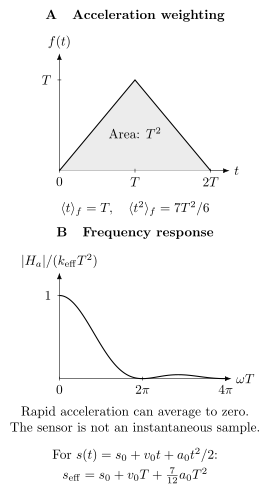
The three-pulse sensor averages acceleration with a triangular kernel. Its area is $T^2$, its mean time is $T$, and its normalized frequency response vanishes at $\omega T=2\pi,4\pi,\ldots$. The final expression uses a quadratic trajectory $s(t)$ to show the corresponding effective position, $s_{\mathrm{eff}}=T^{-2}\int f(t)s(t)\,dt$; this position is relevant when a gravity gradient makes acceleration depend on height.

Periodicity, Priors, and Dynamic Range

The population likelihood is periodic:

$$p(\Phi+2\pi m) = p(\Phi), \qquad m\in\mathbb Z.$$

An ideal acceleration fringe therefore spans

$$\Delta a_{2\pi} = \frac{2\pi}{K_a}.$$

Local Fisher information describes infinitesimal changes around a specified parameter point. Using it to predict a reliable error bar requires local identifiability and a sufficiently localized estimate. It does not solve the global estimation problem. With prior $\pi_0(a)$ and data $D$, a posterior has the schematic form

$$p(a|D) \propto p(D|a)\pi_0(a),$$

and can remain multimodal. Besides shifts by $2\pi/K_a$, one fixed sine fringe has the reflection symmetry $\Phi\mapsto\pi-\Phi$. Two quadratures remove that reflection ambiguity but remain periodic. Chirp locking, quadrature channels, several interrogation times, or a mechanical accelerometer can identify the branch. Those references and preliminary measurements are part of the protocol.

Squeezed readout also requires an accurately known measurement direction. For an error $\delta$ within the squeezed/antisqueezed plane, diagonal quadrature covariance gives

$$V(\delta)=V_-\cos^2\delta+V_+\sin^2\delta.$$

That formula should not be applied automatically to every inertial phase error. Taking $G=-J_y$ in the spin convention used here, $J_{z,\mathrm{out}}=J_z\cos\Phi+J_x\sin\Phi$; away from midfringe, longitudinal fluctuations and covariance also enter:

$$V_{\mathrm{out}}=V_z\cos^2\Phi+V_x\sin^2\Phi +2\operatorname{Cov}_{\mathrm s}(J_z,J_x)\sin\Phi\cos\Phi.$$

The slope changes at the same time. A useful dynamic-range calculation propagates the actual state and detector, including the phase-reference error, rather than using only the minimum quadrature variance.

Quantum Resources for Inertial Phase

Metrological squeezing

For a collective readout with $N$ atoms, define the operational Wineland parameter

$$\xi_R^2 = N \frac{ \operatorname{Var}(J_{z,\mathrm{out}}) }{ |\partial_\Phi \langle J_{z,\mathrm{out}}\rangle|^2 }.$$

At midfringe, the denominator is $|\langle J_x\rangle|^2$. The attained phase variance of the local linear estimator is

$$(\Delta\Phi)^2 = \frac{\xi_R^2}{N}.$$

Thus, for the same inertial response,

$$(\Delta q)^2 = \frac{\xi_R^2}{NK_q^2}.$$

For fixed $N$ spin-$1/2$ constituents and a linear collective generator, $\xi_R^2<1$ beats the ideal unit-contrast separable benchmark. A particular product-state apparatus with contrast $C_{\mathrm{prod}}$ instead has $\xi_{R,\mathrm{prod}}^2=1/C_{\mathrm{prod}}^2$. Its variance ratio to the squeezed protocol is therefore $r=\xi_{R,\mathrm{sq}}^2 C_{\mathrm{prod}}^2$ at equal $N$ and response. An improvement over a degraded product implementation need not by itself violate the ideal separable bound. It includes the contrast penalty through the response slope. Noise squeezing alone, for example

$$\frac{4\operatorname{Var}(J_z)}{N}<1,$$

does not guarantee $\xi_R^2<1$ if coherence is lost.

An enhancement in decibels is commonly reported as

$$G_{\mathrm{dB}} = -10\log_{10}\xi_R^2.$$

A $3\ \mathrm{dB}$ gain halves variance and reduces standard deviation by $\sqrt2$; it does not reduce standard deviation by a factor of two.

Quantum Fisher information

For a pure state encoded by $U_\Phi=e^{-i\Phi G}$,

$$F_Q(\Phi) = 4\operatorname{Var}(G).$$

With the conventional normalization in which each independent two-mode atom has a unit maximum phase Fisher information, separable inputs obey

$$F_Q(\Phi) \leq N.$$

Entangled states can have $F_Q>N$, and ideal maximally correlated states can reach order $N^2$. For inertial parameter $q$,

$$F_Q(q) = K_q^2F_Q(\Phi).$$

This is a local information measure, not an attained error bar. A laboratory still needs a suitable measurement, control of global phase aliases, and robustness to loss and phase diffusion. The moment estimator gives $F_\Phi\ge N/\xi_R^2$ for its regular likelihood; equality requires additional conditions, such as a locally Gaussian shift distribution with constant variance. See Fisher information and Heisenberg scaling for the measurement optimization and global bounds.

Ways to create useful correlations

Several architectures can supply nonclassical matter-wave inputs:

• collisional spin mixing can create twin-Fock or two-mode squeezed states, followed by coherent transfer from internal to momentum modes;
• one-axis twisting can shear a collective uncertainty distribution into a spin-squeezed state;
• cavity-mediated interactions can generate correlations while mode-filtered cavity fields drive or read momentum transitions; and
• quantum nondemolition measurements can condition or feedback-stabilize a reduced collective variance.

The entangled degree of freedom must match the generator and detector. Internal spin squeezing that is lost during momentum mapping does not enhance a spatial interferometer. Conversely, a squeezed momentum population can survive release yet fail to improve the final phase if recombination contrast or readout slope is degraded.

Atom number and observation time

Prepared and detected atoms

At least four atom numbers may differ:

$$N_{\mathrm{load}} \geq N_{\mathrm{prep}} \geq N_{\mathrm{enc}} \geq N_{\mathrm{det}}.$$

$N_{\mathrm{enc}}$ counts atoms that enter the phase-encoding sequence in the declared state. A benchmark using $N_{\mathrm{det}}$ for the correlated protocol but $N_{\mathrm{enc}}$ for the product protocol is mismatched. The comparison must also fix or explicitly charge for momentum transfer, interrogation time, optical control, acceptance probability, and auxiliary references. Cycle time includes loading, preparation, interrogation, and readout.

For independent white cycles, define information rate

$$\mathcal I_q = \frac{F_q}{T_c}.$$

For an estimator with independent white one-cycle errors of standard deviation $\sigma_q$, the averaging-time coefficient is

$$\eta_q = \sigma_q\sqrt{T_c},$$

so that $\sigma_q(\tau)\simeq\eta_q/\sqrt\tau$ over many cycles. It equals $1/\sqrt{\mathcal I_q}$ only for an efficient estimator. A fair information-rate gain is

$$G_{\mathrm{rate}} = \frac{ F_{q,\mathrm{sq}}/T_{c,\mathrm{sq}} }{ F_{q,\mathrm{prod}}/T_{c,\mathrm{prod}} }.$$

A $3\ \mathrm{dB}$ per-shot variance gain is exactly canceled if squeezing doubles the cycle time while all other resources remain equal.

Acceptance and postselection

If a preparation succeeds with probability $q(\theta)$ and both accepted and rejected records are retained, the Fisher information per attempt can be decomposed as

$$F_{\mathrm{tot}} = qF_{\mathrm{acc}} + (1-q)F_{\mathrm{rej}} + \frac{ [\partial_\theta q]^2 }{q(1-q)}.$$

When $q$ is parameter independent and rejected trials carry no information, $F_{\mathrm{tot}}=qF_{\mathrm{acc}}$. Reporting only $F_{\mathrm{acc}}$ overstates performance. The clock continues to run while an entangled state fails to prepare.

Technical-noise crossover

Suppose a matched product state has quantum phase variance $1/N$, a squeezed state has $\xi_R^2/N$, and both share additive technical variance $\sigma_{\mathrm{tech}}^2$. Then

$$\begin{aligned} \sigma_{\Phi,\mathrm{prod}}^2 &= \frac1N+\sigma_{\mathrm{tech}}^2,\\ \sigma_{\Phi,\mathrm{sq}}^2 &= \frac{\xi_R^2}{N} +\sigma_{\mathrm{tech}}^2. \end{aligned}$$

The total variance gain is

$$G_{\mathrm{tot}} = \frac{ N^{-1}+\sigma_{\mathrm{tech}}^2 }{ \xi_R^2N^{-1}+\sigma_{\mathrm{tech}}^2 }.$$

As vibration, laser phase noise, wavefront variation, or detection noise dominates, $G_{\mathrm{tot}}\to1$. Quantum enhancement is most useful after technical noise has been suppressed below or near the independent-atom term.

Loss, Contrast, and Interactions

Particle loss reduces atom number and can destroy correlations. Loss before encoding and missed detection after encoding act at different stages. Their information penalties can coincide in special commuting independent-loss models, but this must be shown for the actual state, encoding, and measurement rather than assumed.

Strongly correlated states have different fragilities. An $N$-atom GHZ-like coherence can be destroyed by one lost atom in a simple loss model, giving a survival factor that scales as

$$P_{\mathrm{coh}} \sim \eta^N.$$

Moderately squeezed states often degrade more gracefully, but their actual gain depends on loss channel, generator, and readout. There is no universal formula obtained by replacing $N$ with $\eta N$.

Interactions can both create squeezing and produce unwanted phase diffusion, density shifts, mode deformation, and expansion. A Bose–Einstein condensate offers low expansion and high mode quality, yet its source cycle can be long and its mean-field dynamics must be controlled. Delta-kick collimation can reduce expansion without being an entanglement resource. Improvements from larger $k_{\mathrm{eff}}$, longer $T$, colder atoms, higher flux, better contrast, or better vibration rejection are valuable but should be named as response or engineering gains rather than attributed to entanglement.

Differential and Rotation Measurements

Gradiometry

Let two interferometers estimate phases $\Phi_1$ and $\Phi_2$. The differential phase is

$$\Delta\Phi = \Phi_2-\Phi_1.$$

Its variance is

$$\operatorname{Var}(\Delta\Phi) = V_1+V_2-2\operatorname{Cov}(\Phi_1,\Phi_2).$$

For independent product states with equal atom number $N$, contrast $C$, and negligible technical noise,

$$\operatorname{Var}(\Delta\Phi)_{\mathrm{SQL}} = \frac{2}{C^2N}.$$

Common optical-phase or vibration noise can produce useful classical covariance and cancel in the difference. Local squeezing can reduce $V_1$ and $V_2$. Entanglement shared between sensor nodes can instead engineer the differential quadrature directly. These strategies have different resource boundaries and robustness; a common-mode rejection ratio is not itself proof of nonclassical enhancement.

For a known, nonzero effective baseline $L_{\mathrm{eff}}$ along the measured gradient component and matched acceleration scale factors,

$$\widehat\Gamma = \frac{ \Delta\Phi-\Delta b }{ k_{\mathrm{eff}}T^2L_{\mathrm{eff}} }.$$

Quantum correlations do not determine $L_{\mathrm{eff}}$ or eliminate leakage from a common acceleration through scale-factor mismatch.

Rotation and multi-axis sensing

Counterpropagating trajectories can generate phases

$$\begin{aligned} \Phi_+ &= K_a a+K_\Omega\Omega+b_+,\\ \Phi_- &= K_a a-K_\Omega\Omega+b_-. \end{aligned}$$

Their sum and difference separate acceleration-like and rotation-like channels only to the extent that scale factors and trajectories match. Squeezing both channels lowers their quantum statistical terms but cannot correct a launch- velocity drift or wavefront asymmetry.

Simultaneous arrays can provide several response vectors in one shot. Their advantage over sequential axis rotation is reduced temporal mismatch, not automatic rank or calibration. A multi-axis quantum-enhancement claim should compare covariance matrices or a declared scalar loss, for example

$$\mathcal L = \operatorname{Tr} \left( \mathbf W \operatorname{Cov}\widehat{\boldsymbol\theta} \right),$$

with positive task-weight matrix $\mathbf W$, rather than selecting the best single diagonal element after the measurement.

Hybrid Quantum–Classical Inertial Sensing

Atom interferometers can provide stable low-frequency references, with systematic corrections still required; many use cyclic readout and have limited capture range. Mechanical accelerometers and optical or electromechanical gyroscopes offer higher bandwidth and dynamic range but can have drifting bias. A hybrid estimator uses both data streams.

The correct statistical object is a joint model such as

$$p \left( n_k,z_{\mathrm{aux}}(t) \mid \boldsymbol\theta, \boldsymbol\lambda \right),$$

where $n_k$ is the atomic output and $z_{\mathrm{aux}}(t)$ is the auxiliary record. Gain, delay, axis orientation, lever arm, saturation, and auxiliary bias belong to $\boldsymbol\lambda$. Filtering the auxiliary record through the atomic sensitivity function predicts the vibration phase and often identifies the fringe branch.

An auxiliary sensor can increase usable information by preserving operation in a dynamic environment. It does not reduce atom projection noise, and it is not free. A quantum-enhancement comparison must give product and entangled protocols access to the same auxiliary record, or count any difference as a resource. Field performance should be judged from the final hybrid output, including cycle slips and bias tracking, not from a quiet subset of atomic shots.

Worked comparison with a finite-contrast reference

Consider a vertical interferometer with

$$\begin{aligned} k_{\mathrm{eff}} &= 1.61\times10^7\ \mathrm{m^{-1}},\\ T &= 0.100\ \mathrm s,\\ N &= 10^6,\\ C &= 0.40,\\ T_c &= 0.50\ \mathrm s. \end{aligned}$$

The ideal scale factor is

$$K_a = k_{\mathrm{eff}}T^2 = 1.61\times10^5\ \frac{\mathrm{rad}} {\mathrm{m\,s^{-2}}}.$$

The independent-atom phase and acceleration baselines are

$$\Delta\Phi_{\mathrm{SQL}} = \frac{1}{C\sqrt N} = 2.50\times10^{-3}\ \mathrm{rad},$$

and

$$\Delta a_{\mathrm{SQL}} = 1.55\times10^{-8}\ \mathrm{m\,s^{-2}}$$

per cycle. The white-noise coefficient is

$$\eta_a = \Delta a_{\mathrm{SQL}}\sqrt{T_c} = 1.10\times10^{-8}\ \mathrm{m\,s^{-2}\,Hz^{-1/2}}.$$

Now suppose the correlated protocol has the operational Wineland parameter $\xi_{R,\mathrm{sq}}^2=10^{-3/10}=0.501$, measured after the complete sequence. This is $3.00\,\mathrm{dB}$ below the unit-contrast independent benchmark. The actual product apparatus above has $\xi_{R,\mathrm{prod}}^2=1/C^2=6.25$. Thus

$$\Delta a_{\mathrm{sq}} =\frac{\sqrt{0.501}}{K_a\sqrt N} =4.40\times10^{-9}\ \mathrm{m\,s^{-2}},$$

and its variance ratio to that product apparatus is $r=0.501 C^2=0.0802$. The contrast penalty is already included in $\xi_R^2$; multiplying the product uncertainty by $\sqrt{\xi_R^2}$ would count it incorrectly.

If preparation doubles the cycle time to $1.00\,\mathrm s$, then

$$\eta_{a,\mathrm{sq}}=4.40\times10^{-9}\ \mathrm{m\,s^{-2}\,Hz^{-1/2}}.$$

This is $0.400$ times the product coefficient, a factor $6.24$ improvement in variance per elapsed time under the independent-noise assumptions. If “3 dB gain” instead meant a variance ratio $r=0.501$ relative to the actual $C=0.40$ implementation, doubling cycle time would essentially cancel it. The two definitions describe different prepared states.

Add $2.0\,\mathrm{mrad}$ RMS independent technical phase noise per cycle to both protocols. The ratio of total one-cycle variances becomes

$$G_{\mathrm{tot}} =\frac{(2.50\,\mathrm{mrad})^2+(2.0\,\mathrm{mrad})^2} {(0.708\,\mathrm{mrad})^2+(2.0\,\mathrm{mrad})^2} =2.28.$$

After the doubled cycle time, the variance-per-time improvement is only $2.28/2=1.14$. Slowly correlated noise would require its time covariance, rather than this independent-cycle formula.

Interferometric gain and systematic uncertainty

Experiments such as Cassens and colleagues’ atomic gravimeter demonstrate the relevant progression from preparing correlated atoms to estimating an inertial quantity. The distinction is physical: the correlations must survive momentum transfer, free evolution, recombination, and detection. For dated results and open instrument challenges, see gravimetry research.

Statistical gain does not remove wavefront, Coriolis, gradient, timing, reference-height, or environmental biases. It can reduce averaging time, which may reduce exposure to drift, but that additional benefit depends on the actual noise process. Differential rejection of shared vibration can also be entirely classical; a separable comparator must have the same access to that common reference.

Exercises

1. Independent-atom acceleration baseline

An interferometer has $k_{\mathrm{eff}}=1.60\times10^7\ \mathrm{m^{-1}}$, $T=80\ \mathrm{ms}$, $N=2.5\times10^5$, and $C=0.60$. Find the ideal one-cycle acceleration standard deviation at midfringe.

Solution

The scale factor is

$$K_a = k_{\mathrm{eff}}T^2 = (1.60\times10^7)(0.080)^2 = 1.024\times10^5\ \frac{\mathrm{rad}}{\mathrm{m\,s^{-2}}}.$$

Since $\sqrt N=500$,

$$\Delta a_{\mathrm{SQL}} = \frac{1}{K_aC\sqrt N} = 3.26\times10^{-8}\ \mathrm{m\,s^{-2}}.$$

2. Convert decibels to averaging-time gain

A squeezed gravimeter reports $-1.7\ \mathrm{dB}$ relative variance. Assume the squeezed and product protocols have equal cycle time and no shared technical noise. Find the variance ratio, standard-deviation ratio, and factor by which the squeezed protocol reaches a fixed statistical variance sooner.

Solution

Let $r$ denote the variance ratio to the stated product comparator. Then

$$r = 10^{-1.7/10} = 0.676.$$

The standard-deviation ratio is

$$\sqrt{r} = 0.822.$$

At equal cycle time, variance falls inversely with averaging time, so the time-to-target improvement is

$$\frac{1}{r} = 1.48.$$

3. Include preparation time

A correlated protocol has $\xi_R^2=0.40$ but takes $1.8$ times as long per cycle as an ideal unit-contrast product-state comparator. Assume Gaussian local phase estimates whose variances attain their information bounds. Find the information-rate gain.

Solution

The per-shot Fisher-information ratio is $1/\xi_R^2=2.5$. The cycle-rate ratio is $1/1.8$, so

$$G_{\mathrm{rate}} = \frac{2.5}{1.8} = 1.39.$$

There remains a wall-time gain, but it is $1.42\ \mathrm{dB}$ rather than the $3.98\ \mathrm{dB}$ per-shot variance gain.

4. Diagnose an unidentifiable two-axis sensor

Two simultaneous channels have response rows

$$\mathbf h_1 = (K,0), \qquad \mathbf h_2 = (2K,0)$$

for parameters $(a_x,a_y)$. Can arbitrary squeezing make both components identifiable?

Solution

No. Each Fisher contribution is proportional to $\mathbf h_j\mathbf h_j^{\mathsf T}$, so

$$\mathbf F \propto \begin{pmatrix} 1&0\\ 0&0 \end{pmatrix}.$$

The matrix has rank one. Squeezing can increase its nonzero eigenvalue but cannot create sensitivity to $a_y$. A channel with a response vector having a nonzero $y$ component is required.

5. Differential phase with correlated noise

Two phase estimates each have variance $V$ and covariance $\rho V$. Find the variance of their difference and interpret $\rho>0$.

Solution

Using the covariance identity,

$$\operatorname{Var}(\Phi_2-\Phi_1) = V+V-2\rho V = 2V(1-\rho).$$

Positive covariance suppresses the differential noise. It may arise from common laser or vibration noise and is not automatically a quantum correlation. Establishing quantum enhancement requires a matched separable network benchmark and a witness or information comparison at the same resource boundary.

6. Technical-noise dilution

Let $N=10^6$, $\xi_R^2=0.25$, and $\sigma_{\mathrm{tech}}=1.5\times10^{-3}\ \mathrm{rad}$. Compute the total variance gain over a product input.

Solution

The product quantum variance is $10^{-6}\ \mathrm{rad^2}$ and the technical variance is $2.25\times10^{-6}\ \mathrm{rad^2}$. Therefore

$$G_{\mathrm{tot}} = \frac{ 1.00\times10^{-6}+2.25\times10^{-6} }{ 0.25\times10^{-6}+2.25\times10^{-6} } = 1.30.$$

The nominal $6.02\ \mathrm{dB}$ quantum variance gain becomes only $10\log_{10}(1.30)=1.14\ \mathrm{dB}$ in the total phase variance.

7. Phase-wrap spacing

For $k_{\mathrm{eff}}=1.61\times10^7\ \mathrm{m^{-1}}$ and $T=0.12\ \mathrm s$, find the acceleration separation between adjacent fringe branches.

Solution

The scale factor is

$$K_a = (1.61\times10^7)(0.12)^2 = 2.3184\times10^5\ \frac{\mathrm{rad}}{\mathrm{m\,s^{-2}}}.$$

Hence

$$\Delta a_{2\pi} = \frac{2\pi}{K_a} = 2.71\times10^{-5}\ \mathrm{m\,s^{-2}}.$$

A much smaller local uncertainty does not identify the correct branch if the prior or auxiliary acceleration error exceeds this scale.

8. Acceleration curvature within one interrogation

Let $a(t)=a_c+j(t-T)+\tfrac12\beta(t-T)^2$ during the ideal three-pulse sequence. Calculate $a_f$ and compare it with the instantaneous acceleration $a(T)=a_c$.

Solution

The triangular kernel is symmetric about $T$, so the odd term integrates to zero. Direct integration gives

$$\frac1{T^2}\int_0^{2T}f(t)(t-T)^2\,dt=\frac{T^2}{6}.$$

Therefore $a_f=a_c+\beta T^2/12$. Linear variation alone gives the midpoint value exactly; curvature changes it. A quieter phase readout reduces random uncertainty in this weighted acceleration, but does not convert the result into an instantaneous sample.

References

• K. Bongs et al., “Taking atom interferometric quantum sensors from the laboratory to real-world applications,” Nature Reviews Physics 1, 731–739 (2019).

• B. Canuel et al., “Six-axis inertial sensor using cold-atom interferometry,” Physical Review Letters 97, 010402 (2006).

• C. Cassens, B. Meyer-Hoppe, E. Rasel, and C. Klempt, “Entanglement-enhanced atomic gravimeter,” Physical Review X 15, 011029 (2025).

• P. Cheiney et al., “Navigation-compatible hybrid quantum accelerometer using a Kalman filter,” Physical Review Applied 10, 034030 (2018).

• A. D. Cronin, J. Schmiedmayer, and D. E. Pritchard, “Optics and interferometry with atoms and molecules,” Reviews of Modern Physics 81, 1051–1129 (2009).

• M. Kasevich and S. Chu, “Atomic interferometry using stimulated Raman transitions,” Physical Review Letters 67, 181–184 (1991).

• J. Lautier et al., “Hybridizing matter-wave and classical accelerometers,” Applied Physics Letters 105, 144102 (2014).

• A. Peters, K. Y. Chung, and S. Chu, “High-precision gravity measurements using atom interferometry,” Metrologia 38, 25–61 (2001).

• L. Pezzè, A. Smerzi, M. K. Oberthaler, R. Schmied, and P. Treutlein, “Quantum metrology with nonclassical states of atomic ensembles,” Reviews of Modern Physics 90, 035005 (2018).

• S. S. Szigeti, S. P. Nolan, J. D. Close, and S. A. Haine, “High-precision quantum-enhanced gravimetry with a Bose–Einstein condensate,” Physical Review Letters 125, 100402 (2020).