Squeezing

Squeezing reduces the fluctuations of a quadrature or collective observable below a specified reference level. For a canonical quadrature squeezed below vacuum noise, the uncertainty relation forces increased noise in its conjugate quadrature. A reduction relative to an arbitrary noisy reference need not have that property: cooling a thermal mode can reduce both quadrature variances. In metrology, the reduced variance is useful only when it is aligned with the signal response and survives preparation, encoding, loss, readout, and estimation.

For a measured observable $M$ and a parameter $\theta$, local error propagation gives

$$(\Delta\theta_M)^2 \simeq \frac{ (\Delta M)^2 }{ \left| \partial_\theta\langle M\rangle \right|^2 }.$$

Reducing $(\Delta M)^2$ helps only if the response $|\partial_\theta\langle M\rangle|$ is not reduced by as much or more. This distinction separates noise squeezing, a statement about a state or data stream, from metrological squeezing, a statement about an estimator under a matched resource boundary.

Required background. Parameter estimation supplies the likelihood and local response; Fisher information connects the response to precision; the standard quantum limit specifies the independent-probe comparison.

Helpful background. Covariance describes correlated fluctuations. Optical preparation and homodyne detection are developed in Squeezed Light; collective-spin criteria are developed in Spin Squeezing.

Variance relative to a reference

Specify the measured observable, the comparison state, and where the noise is measured. Vacuum noise at the detector, thermal noise at the source, and the variance of the final parameter estimate are different comparisons.

Write the normalized variance factor as

$$\xi_M^2 = \frac{ (\Delta M)^2 }{ (\Delta M)^2_{\mathrm{ref}} }.$$

Then $\xi_M^2<1$ means that $M$ is variance-squeezed relative to that reference. It does not yet say that the state is nonclassical, entangled, or metrologically superior. Those conclusions require additional properties of the reference and task.

For noise power or variance, the signed decibel level is

$$L_{\mathrm{dB}} = 10\log_{10}\xi_M^2.$$

Squeezing lies below zero on this scale. Experimental prose often quotes the positive magnitude

$$S_{\mathrm{dB}} = -10\log_{10}\xi_M^2.$$

Thus $3\ \mathrm{dB}$ of squeezing means approximately one-half the reference variance, not one-half the standard deviation.

Uncertainty Is Redistributed

For Hermitian observables $A$ and $B$, define the symmetrized covariance

$$\operatorname{Cov}(A,B) = \frac12 \langle \{\Delta A,\Delta B\} \rangle.$$

The Robertson–Schrödinger relation is

$$(\Delta A)^2(\Delta B)^2 - \operatorname{Cov}(A,B)^2 \ge \frac14 \left| \langle[A,B]\rangle \right|^2.$$

For canonical quadratures with a fixed commutator, squeezing one direction below vacuum noise therefore does not erase quantum uncertainty. In an ideal pure Gaussian state it increases the orthogonal variance so that the determinant of the covariance matrix remains at its minimum. Loss, thermal noise, and imperfect preparation usually increase the determinant as well.

For a two-component observable vector

$$\mathbf X = \begin{pmatrix} X_1\\ X_2 \end{pmatrix},$$

the covariance matrix is

$$V_{jk} = \frac12 \langle \{\Delta X_j,\Delta X_k\} \rangle.$$

The variance along a unit direction $\mathbf w$ is

$$\operatorname{Var}(\mathbf w^{\mathsf T}\mathbf X) = \mathbf w^{\mathsf T}V\mathbf w.$$

The principal axes are the eigenvectors of $V$. A small eigenvalue is useful only if the parameter moves the mean, or changes another measured statistic, in a direction that the readout can exploit.

Metrological Squeezing

Let the reference protocol have observable $M_0$, variance $(\Delta M_0)^2$, and response

$$s_0 = \left| \partial_\theta \langle M_0\rangle \right|.$$

For a candidate squeezed protocol with response $s$, define

$$\xi_{\mathrm{met}}^2 = \frac{ (\Delta M)^2/s^2 }{ (\Delta M_0)^2/s_0^2 }.$$

When both error-propagation models are calibrated and locally valid,

$$\xi_{\mathrm{met}}^2<1$$

means smaller parameter variance than the reference. The variance gain is

$$G = \frac{1}{\xi_{\mathrm{met}}^2},$$

or $10\log_{10}G$ decibels.

This ratio exposes a common failure mode. A preparation may reduce noise by a factor of four while reducing contrast, coherence, or slope by a factor of three. Its parameter variance is then worse by a factor $4^{-1}\times3^2=9/4$ despite the visibly quieter readout.

The reference must be the best allowed unsqueezed strategy under the same probe count, sample exposure, duration, bandwidth, efficiency, prior, and accepted-run rule. Beating a deliberately weak coherent or product-state implementation is not the same as beating the standard quantum limit.

Signal–Noise Geometry

Suppose a jointly measured classical vector $\mathbf X$ has a Gaussian distribution with mean $\boldsymbol\mu_\theta$ and positive-definite, parameter-independent covariance $V$. Near an operating point, define the response vector

$$\mathbf d = \partial_\theta \boldsymbol\mu_\theta.$$

A linear readout

$$Y = \mathbf w^{\mathsf T}\mathbf X$$

has local Fisher information

$$F_C(\mathbf w) = \frac{ (\mathbf w^{\mathsf T}\mathbf d)^2 }{ \mathbf w^{\mathsf T}V\mathbf w }.$$

The Cauchy–Schwarz inequality in the $V$ metric gives

$$F_C(\mathbf w) \le \mathbf d^{\mathsf T}V^{-1}\mathbf d,$$

with equality for

$$\mathbf w_{\mathrm{opt}} \propto V^{-1}\mathbf d.$$

This result is the cleanest statement of useful alignment. The optimal readout is not generally parallel to the signal displacement; it weights components by their inverse covariance. If the covariance also depends on $\theta$, the full Gaussian Fisher information contains an additional term,

$$F_C = \mathbf d^{\mathsf T}V^{-1}\mathbf d + \frac12 \operatorname{Tr} \left[ V^{-1}(\partial_\theta V) V^{-1}(\partial_\theta V) \right].$$

Variance-only error propagation misses information carried by a changing noise ellipse. These are classical Gaussian likelihood formulas. For noncommuting quantum quadratures, one cannot assume that their bare state covariance is available as a simultaneous measurement record: a joint detector generally adds noise. Alternatively, measure the single chosen quadrature $\mathbf w^{\mathsf T}\mathbf X$ on each copy, with its own response and variance.

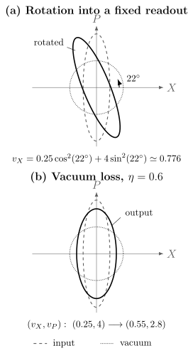
Ellipse semiaxes are standard deviations, in units of the vacuum standard deviation. The input variances are $(v_X,v_P)=(0.25,4)$, whose product is one. (a) Rotation by $22^\circ$ increases the variance projected onto the fixed $X$ readout. (b) Pure loss with $\eta=0.6$ changes the variances to $(0.55,2.8)$. It also attenuates a previously encoded mean displacement by $\sqrt{\eta}$, so the noise change alone is not the metrological gain.

Angle Error and Anti-Squeezed Leakage

Let the principal normalized variances be $v_-=e^{-2r}$ and $v_+=e^{2r}$. If the readout is misaligned from the squeezed axis by an angle $\delta$, the measured variance is

$$v(\delta) = v_-\cos^2\delta + v_+\sin^2\delta.$$

For a random zero-mean angle error with small variance $\sigma_\delta^2$,

$$\mathbb E[v] \simeq v_- + (v_+-v_-) \sigma_\delta^2.$$

Stronger source squeezing therefore raises the phase-control requirement: the anti-squeezed variance grows exponentially and can dominate even through a small angular leak. “More squeezing” is not monotonic improvement when the readout phase is noisy. For Gaussian angle jitter $\delta\sim\mathcal N(0,\sigma_\delta^2)$ the exact averaged variance is

$$\mathbb E[v] =\frac{1+u}{2}e^{-2r}+\frac{1-u}{2}e^{2r}, \qquad u=e^{-2\sigma_\delta^2}.$$

This follows from $\mathbb E[\cos(2\delta)]=u$. Exercise 8 minimizes this noise; optimizing a complete sensor also requires the jitter-averaged signal response.

The same geometry appears for collective spins. A fluctuating rotation axis, local-oscillator phase, or nonlinear readout maps anti-squeezed fluctuations into the estimator. Covariance must be propagated through the actual control sequence, not attached to a nominal axis at state-preparation time.

Optical Quadrature Example

For one bosonic mode, use

$$X = \frac{a+a^\dagger}{\sqrt2}, \qquad P = \frac{a-a^\dagger}{i\sqrt2}, \qquad [X,P]=i.$$

The vacuum variances are $1/2$. In one phase convention, an ideal squeezed vacuum has

$$(\Delta X)^2 = \frac12e^{-2r}, \qquad (\Delta P)^2 = \frac12e^{2r}.$$

For phase sensing, rotate the squeezing ellipse by $\pi/2$ so that $(\Delta P)^2=e^{-2r}/2$ instead. Add a real displacement $\alpha$ and encode a small phase $\phi$ relative to an external phase reference. At the operating point the mean phase-quadrature response is

$$\partial_\phi\langle P\rangle \simeq \sqrt2\,|\alpha|.$$

Phase-quadrature squeezing then gives

$$\Delta\phi \simeq \frac{e^{-r}}{2|\alpha|} = \frac{e^{-r}}{2\sqrt{n_{\mathrm c}}},$$

where $n_{\mathrm c}=|\alpha|^2$ is the coherent displacement energy in this simple model. The formula is local and assumes ideal alignment and readout. It does not charge the squeezed-vacuum energy

$$n_{\mathrm s} = \sinh^2r,$$

source pump, loss, or phase reference.

See Squeezed Light for mode definitions, generation, homodyne spectra, and the distinction between source and observed noise.

Collective-Spin Preview

For $N$ effective spin-$1/2$ probes, define

$$J_k = \frac12 \sum_{j=1}^{N} \sigma_k^{(j)}.$$

A coherent spin state polarized along $x$ has

$$|\langle\mathbf J\rangle| = \frac N2, \qquad (\Delta J_y)^2 = (\Delta J_z)^2 = \frac N4.$$

The Kitagawa–Ueda noise-squeezing parameter is

$$\xi_S^2 = \frac{ 4\min_{\perp}(\Delta J_\perp)^2 }{N}.$$

It compares the narrowest transverse spin variance with coherent-spin noise. The Wineland metrological parameter includes the response or contrast:

$$\xi_R^2 = \frac{ N\min_{\perp}(\Delta J_\perp)^2 }{ |\langle\mathbf J\rangle|^2 }.$$

For a suitable small-angle Ramsey readout,

$$(\Delta\phi)^2 = \frac{\xi_R^2}{N}.$$

It is possible to have $\xi_S^2<1$ but little useful mean spin, so $\xi_R^2$ is the relevant local spectroscopic metric. For a fixed number of spin-$1/2$ constituents, every fully separable state satisfies $\xi_R^2\ge1$; thus $\xi_R^2<1$ certifies entanglement between those constituents. Permutation symmetry is not required for this witness. The converse fails: many entangled states are not spin-squeezed by this criterion, and some have metrological value requiring a nonlinear measurement.

One-axis twisting, two-axis countertwisting, collisional dynamics, cavity feedback, and quantum-nondemolition measurement can generate collective-spin squeezing. Their detailed scaling, entanglement depth, curvature, phase range, and clock implementation require a dedicated treatment; the formulas above serve only to distinguish variance squeezing from response-aware gain.

Differential and Multimode Squeezing

Squeezing need not reduce the marginal variance of one subsystem. For two readouts $X_A$ and $X_B$,

$$\operatorname{Var}(X_A-X_B) = \operatorname{Var}(X_A) + \operatorname{Var}(X_B) - 2\operatorname{Cov}(X_A,X_B).$$

Positive correlations can make the difference quieter than its independent-readout reference. This structure underlies twin-beam intensity-difference squeezing, EPR-like quadratures, differential clock comparisons, and distributed sensing.

The reference must follow the same mode transformation. Comparing a joint observable with the single-mode vacuum variance gives the wrong normalization. Likewise, common-mode technical-noise rejection can produce a quiet difference channel without nonclassical squeezing. A nonclassical or entanglement claim needs the appropriate separability or classical-state bound, not merely a low measured variance.

Loss, Thermal Noise, and Efficiency

Normalize each quadrature variance so that vacuum is one. Mixing a mode with an independent environment on a beam splitter of intensity transmissivity $\eta$ gives

$$V_{\mathrm{out}}=\eta V_{\mathrm{in}}+(1-\eta)V_{\mathrm{env}}, \qquad \mathbf d_{\mathrm{out}}=\sqrt{\eta}\,\mathbf d_{\mathrm{in}}.$$

For vacuum, $V_{\mathrm{env}}=I$ and $v_{\mathrm{out}}=\eta v_{\mathrm{in}}+1-\eta$. Even infinite input squeezing leaves the floor $1-\eta$. For a thermal environment, $V_{\mathrm{env}}=(2n_{\mathrm{th}}+1)I$: the environmental noise is weighted by the lost fraction, rather than added independently of it.

Optical propagation loss and detector inefficiency often admit this vacuum attenuator model. Mode mismatch adds vacuum only when the other sampled modes are empty. Thermal microwave or mechanical environments add thermal noise. Atomic loss, contrast decay, and imperfect readout transfer require their own state and response models; they cannot all be identified with one bosonic vacuum-loss efficiency.

Conditional and Unconditional Squeezing

A preparation measurement can reduce the variance of a later observable $M$ conditional on a retained record $R$. For the corresponding joint distribution, the law of total variance gives

$$\operatorname{Var}(M) =\mathbb E_R[\operatorname{Var}(M\mid R)] +\operatorname{Var}_R(\mathbb E[M\mid R]).$$

Thus the average conditional variance is smaller, although an individual outcome need not be narrower than the unconditional distribution. Discarding $R$ mixes different conditional means. Feedback that removes those random means can turn conditional squeezing into deterministic squeezing, as in the collective-measurement experiment of Cox and colleagues.

Keeping every preparation record differs from accepting only selected records. Postselection requires counting all attempts and including information in the acceptance probability. In either case, preparation and sensing records may be correlated: use their joint likelihood rather than adding independent error bars without justification.

Squeezing and Fisher Information

For a one-dimensional Gaussian readout with parameter-dependent mean and fixed variance,

$$F_C = \frac{ (\partial_\theta\langle M\rangle)^2 }{ (\Delta M)^2 }.$$

The error-propagation variance is exactly $1/F_C$ in this local model. Squeezing improves the implemented Fisher information when it reduces the denominator without sacrificing the numerator.

The quantum Fisher information optimizes over all POVMs on the encoded state; a restricted detector may not attain it. A squeezed quadrature can make a simple homodyne, population, or linear detector nearly optimal, but variance squeezing is neither necessary nor sufficient for maximizing QFI. Non-Gaussian states may carry information in higher moments; a squeezed state measured on the wrong axis may leave most of its QFI inaccessible.

For $N$ spin-$1/2$ constituents under a collective rotation with generator $J_k$, $F_Q>N$ certifies entanglement and sub-SQL potential, while $\xi_R^2<1$ certifies that a specific mean-spin readout can realize such a gain. The QFI criterion is broader; the squeezing criterion is more tied to an operationally simple measurement.

Constant Gain Versus Scaling Gain

If a bright probe has $n_{\mathrm c}\propto N$ and the squeezing strength $r$ is held fixed, then

$$\Delta\theta \propto \frac{e^{-r}}{\sqrt N}.$$

The sensor has a constant sub-SQL factor but retains the $N^{-1/2}$ exponent. This can be extremely valuable: $10\ \mathrm{dB}$ of realized variance gain ideally replaces a factor of ten in averaging resource. It is not Heisenberg scaling.

To make the same local formula behave as $1/N$, one would need

$$e^{-r} \propto N^{-1/2},$$

so $r$ grows logarithmically. But then

$$n_{\mathrm s} = \sinh^2r \;=\;O(N)$$

under this scaling; specifically, $e^{2r}=N$ gives $n_{\mathrm s}\sim N/4$. The squeezed field itself carries an extensive resource and becomes increasingly vulnerable to loss and phase error. A claim based only on the bright displacement $n_{\mathrm c}$ omits that cost.

Optimized lossless interferometers can use coherent displacement and squeezed vacuum together to approach inverse-total-energy scaling. Any such statement must specify total photons, phase reference, estimator range, and whether preparation or rejected events are charged. Under fixed nonzero loss, the asymptotic gain is generally bounded to a constant for standard independent loss models.

Exercises

1. Minimum-uncertainty redistribution

An ideal mode has variances

$$(\Delta X)^2 = \frac12e^{-2r}, \qquad (\Delta P)^2 = \frac12e^{2r}.$$

Verify the uncertainty product and find the variance squeezing in decibels for $r=0.5$.

Solution

The product of variances is

$$(\Delta X)^2(\Delta P)^2 = \frac14,$$

so $\Delta X\Delta P=1/2$. Relative to vacuum, the squeezed variance factor is $e^{-2r}=e^{-1}$. Its positive squeezing magnitude is

$$S_{\mathrm{dB}} = -10\log_{10}(e^{-1}) \approx 4.34\ \mathrm{dB}.$$

2. Optimal linear readout

For a Gaussian measurement vector with covariance $V\succ0$ and response $\mathbf d$, show that

$$\frac{(\mathbf w^{\mathsf T}\mathbf d)^2} {\mathbf w^{\mathsf T}V\mathbf w} \le \mathbf d^{\mathsf T}V^{-1}\mathbf d.$$

Solution

Write

$$\mathbf w^{\mathsf T}\mathbf d = (V^{1/2}\mathbf w)^{\mathsf T} (V^{-1/2}\mathbf d).$$

Cauchy–Schwarz gives

$$(\mathbf w^{\mathsf T}\mathbf d)^2 \le (\mathbf w^{\mathsf T}V\mathbf w) (\mathbf d^{\mathsf T}V^{-1}\mathbf d).$$

Dividing by the positive readout variance proves the bound. Equality requires $V^{1/2}\mathbf w\propto V^{-1/2}\mathbf d$, or $\mathbf w\propto V^{-1}\mathbf d$.

3. Angle leakage

A state has $10\ \mathrm{dB}$ squeezing and $15\ \mathrm{dB}$ anti-squeezing in variance. Find the measured normalized variance at a fixed angle error $\delta=3^\circ$.

Solution

The principal variances are

$$v_- = 10^{-10/10} = 0.1, \qquad v_+ = 10^{15/10} \approx 31.62.$$

Therefore

$$\begin{aligned} v(3^\circ) &= 0.1\cos^2(3^\circ) +31.62\sin^2(3^\circ) \\ &\approx 0.186. \end{aligned}$$

The observed squeezing is

$$-10\log_{10}(0.186) \approx 7.30\ \mathrm{dB}.$$

A small angle error has discarded about $2.7\ \mathrm{dB}$ because the anti-squeezed variance is large.

4. Loss ceiling

An input has normalized variance $v_{\mathrm{in}}=0.10$ and total efficiency $\eta=0.80$. Find the output variance and observed squeezing. What is the best possible observed squeezing at that efficiency?

Solution

Pure loss gives

$$v_{\mathrm{out}} = 0.80(0.10)+0.20 = 0.28.$$

Thus

$$S_{\mathrm{obs}} = -10\log_{10}(0.28) \approx 5.53\ \mathrm{dB}.$$

As $v_{\mathrm{in}}\to0$, the output approaches $1-\eta=0.20$, corresponding to a ceiling of

$$-10\log_{10}(0.20) \approx 6.99\ \mathrm{dB}.$$

5. Noise squeezing versus metrological squeezing

A preparation reduces readout variance to $0.40$ of the reference but also reduces the signal slope to $0.60$ of the reference. Compute $\xi_{\mathrm{met}}^2$.

Solution

The error-propagation variance ratio is

$$\xi_{\mathrm{met}}^2 = \frac{0.40}{0.60^2} \approx 1.11.$$

Although the observable is noise-squeezed, the parameter estimate is about $11\%$ worse in variance because the response loss is larger.

6. Spin contrast penalty

An $N$-atom state has minimum transverse variance $(\Delta J_\perp)^2=0.10N$ and mean-spin length $|\langle\mathbf J\rangle|=0.30N$. Find $\xi_S^2$ and $\xi_R^2$. Is the state metrologically squeezed by the Wineland criterion?

Solution

The noise parameter is

$$\xi_S^2 = \frac{4(0.10N)}{N} = 0.40.$$

The response-aware parameter is

$$\xi_R^2 = \frac{N(0.10N)}{(0.30N)^2} = \frac{0.10}{0.09} \approx 1.11.$$

The transverse variance is squeezed, but the reduced mean-spin contrast removes the local spectroscopic gain.

7. Correlation-squeezed difference

Two readouts have equal variance $V$ and covariance $cV$. Find the variance of $X_A-X_B$. For what $c$ is the difference variance below the independent reference $2V$?

Solution

Using the covariance identity,

$$\operatorname{Var}(X_A-X_B) = 2V-2cV = 2V(1-c).$$

It is below $2V$ whenever $c>0$. This establishes a quieter difference channel, not by itself nonclassicality or entanglement; a classical common fluctuation can also produce positive covariance.

8. Best squeezing strength with Gaussian angle jitter

For $\delta\sim\mathcal N(0,\sigma_\delta^2)$ with $\sigma_\delta>0$, find the nonnegative squeezing strength $r$ that minimizes the averaged normalized quadrature noise. Give the minimum for small $\sigma_\delta$.

Solution

With $u=e^{-2\sigma_\delta^2}$, differentiating $[(1+u)e^{-2r}+(1-u)e^{2r}]/2$ gives

$$e^{4r_*}=\frac{1+u}{1-u}, \qquad r_*=\frac14\log\frac{1+u}{1-u}.$$

The second derivative is positive. At the minimum the two exponential terms are equal, and

$$\mathbb E[v]_{\min}=\sqrt{1-u^2} =\sqrt{1-e^{-4\sigma_\delta^2}} \simeq 2\sigma_\delta.$$

Stronger squeezing beyond $r_*$ increases the observed noise because the anti-squeezed contribution dominates. This minimizes noise at a fixed jitter distribution; a metrological optimization must also propagate the mean signal and count preparation resources.

References

• C. M. Caves, “Quantum-mechanical noise in an interferometer,” Physical Review D 23, 1693–1708 (1981), doi:10.1103/PhysRevD.23.1693.
• K. C. Cox, G. P. Greve, J. M. Weiner, and J. K. Thompson, “Deterministic squeezed states with collective measurements and feedback,” Physical Review Letters 116, 093602 (2016), doi:10.1103/PhysRevLett.116.093602.
• M. Kitagawa and M. Ueda, “Squeezed spin states,” Physical Review A 47, 5138–5143 (1993), doi:10.1103/PhysRevA.47.5138.
• J. Ma, X. Wang, C. P. Sun, and F. Nori, “Quantum spin squeezing,” Physics Reports 509, 89–165 (2011), doi:10.1016/j.physrep.2011.08.003.
• L. Pezzè, A. Smerzi, M. K. Oberthaler, R. Schmied, and P. Treutlein, “Quantum metrology with nonclassical states of atomic ensembles,” Reviews of Modern Physics 90, 035005 (2018), doi:10.1103/RevModPhys.90.035005.
• O. Pinel, P. Jian, N. Treps, C. Fabre, and D. Braun, “Quantum parameter estimation using general single-mode Gaussian states,” Physical Review A 88, 040102(R) (2013), doi:10.1103/PhysRevA.88.040102.
• H. P. Robertson, “The uncertainty principle,” Physical Review 34, 163–164 (1929), doi:10.1103/PhysRev.34.163.
• E. Schrödinger, “Zum Heisenbergschen Unschärfeprinzip,” Sitzungsberichte der Preussischen Akademie der Wissenschaften, Physikalisch-mathematische Klasse 14, 296–303 (1930), English translation.
• A. Sørensen, L.-M. Duan, J. I. Cirac, and P. Zoller, “Many-particle entanglement with Bose–Einstein condensates,” Nature 409, 63–66 (2001), doi:10.1038/35051038.
• C. Weedbrook et al., “Gaussian quantum information,” Reviews of Modern Physics 84, 621–669 (2012), doi:10.1103/RevModPhys.84.621.
• D. J. Wineland, J. J. Bollinger, W. M. Itano, F. L. Moore, and D. J. Heinzen, “Spin squeezing and reduced quantum noise in spectroscopy,” Physical Review A 46, R6797–R6800 (1992), doi:10.1103/PhysRevA.46.R6797.