Dressed States

A dressed state is an eigenstate of a Hamiltonian that includes both a matter system and its coherent coupling to a field. The word “dressed” emphasizes that the interaction changes both the energies and the state vectors. The eigenstates are no longer bare atomic states, and, when the field is quantized, they are generally not product states of an atom and a definite photon number.

For the standard near-resonant two-state Hamiltonian,

$$H_{\mathrm{RWA}} = \frac{\hbar}{2} \left[ \Delta\sigma_z + \Omega \left( \cos\phi\,\sigma_x + \sin\phi\,\sigma_y \right) \right],$$

the dressed-state separation is

$$\hbar\Omega_R, \qquad \Omega_R = \sqrt{ \Delta^2+\Omega^2 }.$$

The same square-root spectrum appears in one excitation manifold of the Jaynes–Cummings model, with the replacement

$$\Omega \longleftrightarrow 2g\sqrt N.$$

That resemblance is powerful, but it must be interpreted carefully. A semiclassical rotating-frame eigenstate, a joint atom–photon eigenstate, and a Floquet mode are related descriptions, not literally the same object.

Required background. Two-Level Atom fixes the rotating-frame Hamiltonian; Rabi Oscillations explains coherent population transfer; Tensor Products and the Oscillator Ladder Operators supply joint states and photon-number matrix elements.

Three Meanings of Field Dressing

The phrase “atom plus photons” is often used before the field model has been declared. Three common constructions should be separated.

Semiclassical RWA. The state space is the atomic Hilbert space, and the stationary object is a rotating-frame eigenvector. There is no extra field index.

Classical periodic drive. Floquet analysis extends the atomic space by Fourier harmonics. The stationary object is a Floquet mode, and the extra integer labels a harmonic or quasienergy zone.

Quantized single mode. The state space is the atomic Hilbert space tensored with oscillator Fock space. The stationary object is a joint atom–mode eigenvector, and the extra integer is a physical mode occupation.

For a prescribed classical drive, the source is not a quantum subsystem of the model. The rotating-frame dressed vectors live only in the matter Hilbert space. A Floquet construction introduces a Fourier index, sometimes drawn as a photon ladder, but that index is bookkeeping in an extended space.

For a quantized cavity mode, by contrast, $|g,n\rangle$ and $|e,n\rangle$ are physical tensor-product states. Their superpositions can entangle the atom with the mode, and photon-number fluctuations can produce dynamics with no deterministic classical-drive counterpart.

These descriptions agree in overlapping limits. They answer different questions outside those limits.

Semiclassical Dressed States

Detuning, phase, and basis

Use bare matter states satisfying

$$H_0|g\rangle = E_g|g\rangle, \qquad H_0|e\rangle = E_e|e\rangle,$$

with

$$\hbar\omega_0 = E_e-E_g > 0.$$

The drive has angular frequency $\omega_L$, phase $\phi$, and atom-minus-laser detuning

$$\Delta = \omega_0-\omega_L.$$

Thus red detuning means $\Delta>0$. In the ordered basis $(|e\rangle,|g\rangle)$, after removing a common quasienergy, use

$$H_{\mathrm{RWA}} = \frac{\hbar}{2} \begin{pmatrix} \Delta & \Omega e^{-i\phi} \\ \Omega e^{i\phi} & -\Delta \end{pmatrix},$$

where $\Omega\ge0$. Frequency variables are angular frequencies; decay rates are inverse times. The two-level and rotating-wave approximations require the relevant coupling, detuning, and envelope bandwidth to be small compared with the optical sum frequency and the separation from excluded resonances.

Changing the sign convention for $\Delta$, reversing the basis order, or absorbing $\phi$ into a bare state changes the displayed formulas. It does not change consistently computed gaps or probabilities.

Mixing angle

Define

$$\Omega_R = \sqrt{ \Delta^2+\Omega^2 }$$

and choose a mixing angle in the range $0\le\theta\le\pi$ through

$$\cos\theta = \frac{\Delta}{\Omega_R}, \qquad \sin\theta = \frac{\Omega}{\Omega_R}.$$

For a nonzero gap, this definition remains unambiguous on both sides of resonance. The normalized eigenvectors may be chosen as

$$\begin{aligned} |+\rangle &= \cos\frac{\theta}{2}|e\rangle + e^{i\phi} \sin\frac{\theta}{2}|g\rangle, \\ |-\rangle &= - \sin\frac{\theta}{2}|e\rangle + e^{i\phi} \cos\frac{\theta}{2}|g\rangle. \end{aligned}$$

They satisfy

$$H_{\mathrm{RWA}}|\pm\rangle = \varepsilon_\pm|\pm\rangle, \qquad \varepsilon_\pm = \pm \frac{\hbar\Omega_R}{2}.$$

An overall phase on either eigenvector is arbitrary. The relative phase inside a dressed state is not arbitrary once the phases of the bare basis and drive have been fixed.

Bare-state content

The excited-state weights are

$$\begin{aligned} |\langle e|+\rangle|^2 &= \frac12 \left( 1+\frac{\Delta}{\Omega_R} \right), \\ |\langle e|-\rangle|^2 &= \frac12 \left( 1-\frac{\Delta}{\Omega_R} \right). \end{aligned}$$

The corresponding ground-state weights are obtained by subtraction from one. Equivalently,

$$\langle\pm|\boldsymbol\sigma|\pm\rangle = \pm \frac1{\Omega_R} \left( \Omega\cos\phi, \Omega\sin\phi, \Delta \right).$$

Each dressed state points along or opposite the effective field on the Bloch sphere.

On resonance,

$$\Delta=0, \qquad \theta=\frac{\pi}{2},$$

so the states are equal-weight superpositions:

$$|\pm\rangle = \frac1{\sqrt2} \left( |e\rangle \pm e^{i\phi}|g\rangle \right),$$

up to an overall phase and the sign convention used to label the branches. The gap is $\hbar\Omega$.

For large positive detuning,

$$\Delta\gg\Omega,$$

the upper state becomes excited-like and the lower state becomes ground-like. For large negative detuning, their bare character is exchanged. A branch label such as “ground-like” is therefore local in parameter space; the fixed labels $+$ and $-$ denote upper and lower quasienergies within this selected RWA block; they are not a global ordering of all equivalent Floquet-zone representatives.

Inverting the transformation

The bare states can be expanded in the dressed basis:

$$\begin{aligned} |e\rangle &= \cos\frac{\theta}{2}|+\rangle - \sin\frac{\theta}{2}|-\rangle, \\ e^{i\phi}|g\rangle &= \sin\frac{\theta}{2}|+\rangle + \cos\frac{\theta}{2}|-\rangle. \end{aligned}$$

This inverse relation explains resonant Rabi flopping. A suddenly prepared bare state is generally a coherent superposition of two stationary dressed states. Their relative phase evolves at $\Omega_R$, and transforming back to the bare basis produces population oscillation.

The dressed-state picture and the Bloch-sphere picture are therefore not competing explanations. One emphasizes stationary eigenvectors and phase accumulation; the other emphasizes precession about the same effective Hamiltonian vector.

Avoided Crossings

With $\Omega=0$, the rotating-frame bare quasienergies are

$$\varepsilon_e^{(0)} = +\frac{\hbar\Delta}{2}, \qquad \varepsilon_g^{(0)} = -\frac{\hbar\Delta}{2}.$$

They cross at $\Delta=0$. A nonzero coupling replaces this crossing by

$$\varepsilon_\pm = \pm \frac{\hbar}{2} \sqrt{ \Delta^2+\Omega^2 },$$

whose minimum separation is

$$\left. \varepsilon_+-\varepsilon_- \right|_{\Delta=0} = \hbar\Omega.$$

An avoided crossing records two facts at once:

• the eigenvalues repel because the states are coupled;
• the eigenvectors exchange their bare-state character across resonance.

The second fact is easy to miss if only the energy curves are plotted. Hellmann–Feynman differentiation exposes it:

$$\frac{\partial\varepsilon_\pm}{\partial\Delta} = \frac{\hbar}{2} \langle\pm|\sigma_z|\pm\rangle = \pm \frac{\hbar\Delta}{2\Omega_R}.$$

Far from resonance, a branch slope approaches the slope of one bare state. At resonance both slopes vanish because each branch contains equal bare weight.

The avoided-crossing plot and exact far-detuned expansion are developed for light shifts on AC Stark Shift. The important lesson here is about basis identity: following an eigenvalue continuously is not the same operation as holding a bare label fixed.

Preparing and Reading a Dressed State

Sudden turn-on

Suppose the system begins in $|g\rangle$ and a constant drive is switched on much faster than $1/\Omega_R$. The state does not instantaneously rotate into an eigenvector. Immediately after the switch it is still $|g\rangle$, which is a superposition of $|+\rangle$ and $|-\rangle$. Subsequent interference produces Rabi oscillations.

This is a quench into the dressed basis, not preparation of one dressed state.

Adiabatic turn-on

If $\Omega(t)$ and $\Delta(t)$ change slowly while the dressed gap stays open, an initial instantaneous eigenstate follows its branch up to dynamical and geometric phases. For the phase-fixed two-state model,

$$\dot\theta = \frac{ \Delta\dot\Omega-\Omega\dot\Delta }{ \Omega_R^2 },$$

and a useful local condition is

$$|\dot\theta| \ll \Omega_R.$$

The off-diagonal coupling in the instantaneous dressed basis is proportional to $\dot\theta/2$. For a varying phase the magnitude is instead $\tfrac12\sqrt{\dot\theta^2+\sin^2\theta\,\dot\phi^2}$. Compare it with $\Omega_R$. These are local diagnostics: the full ramp history and duration also matter, because small transitions can accumulate resonantly.

At exact resonance, turning on from $\Omega=0$ begins at a degeneracy. There is then no unique resonant dressed branch for the ordinary nondegenerate adiabatic theorem to select. A finite initial detuning, an explicit symmetry-breaking term, or a deliberately prepared superposition is needed to define the outcome.

For a linear sweep

$$\Delta(t) = vt, \qquad \Omega(t) = \Omega,$$

the ideal infinite-time Landau–Zener probability to remain on the same diabatic branch is

$$P_{\mathrm{diab}} = \exp \left( - \frac{\pi\Omega^2}{2|v|} \right).$$

For finite-time corrections and the derivation, see Landau–Zener Transition.

Switch-off and basis mapping

An abrupt switch-off leaves the state unchanged during the ideal sudden step. A subsequent bare-state measurement samples its bare-basis probabilities; the switch itself is not a projection measurement. An adiabatic switch-off maps each dressed branch onto the bare state it approaches, provided the chosen path ends at nonzero detuning so the gap does not close. These protocols answer different experimental questions:

• sudden release measures the instantaneous bare-state composition;
• adiabatic release measures branch population;
• a phase-controlled ramp can convert dressed coherence into a bare-state population signal.

Statements such as “the atom is half excited” are incomplete unless the switch-off and measurement protocol are specified.

Quantized Mode: Atom Plus Photons

The Jaynes–Cummings manifold gives a concrete example of quantized field dressing. For the derivation from the quantum Rabi interaction, exact propagator, number-statistics dependence, and collapse and revival, see the Jaynes–Cummings Model.

The near-resonant two-level, single-mode Hamiltonian is

$$H_{\rm JC}=\hbar\omega_c a^\dagger a+ \frac{\hbar\omega_0}{2}\sigma_z+ \hbar g(a\sigma_++a^\dagger\sigma_-),$$

where a phase convention makes $g\ge0$. The conserved excitation number $\mathcal N=a^\dagger a+\sigma_+\sigma_-$ selects, for $N\ge1$, the pair $|e,N-1\rangle$, $|g,N\rangle$. Notice that $N$ is total excitation, not the photon number of both components. With $\Delta_c=\omega_0-\omega_c$, this pair has matrix

$$H_N=\hbar\omega_c(N-\tfrac12)\mathbb I+ \frac{\hbar}{2} \begin{pmatrix}\Delta_c&2g\sqrt N\\2g\sqrt N&-\Delta_c\end{pmatrix}.$$

Thus the mixing-angle construction above applies with $\Omega\mapsto2g\sqrt N$ and $\Delta\mapsto\Delta_c$:

$$\begin{aligned} \Omega_N&=\sqrt{\Delta_c^2+4g^2N},\qquad \cos\theta_N=\Delta_c/\Omega_N,\\ |N,+\rangle&=\cos(\theta_N/2)|e,N-1\rangle +\sin(\theta_N/2)|g,N\rangle,\\ |N,-\rangle&=-\sin(\theta_N/2)|e,N-1\rangle +\cos(\theta_N/2)|g,N\rangle,\\ E_{N,\pm}&=\hbar\omega_c(N-\tfrac12)\pm\hbar\Omega_N/2. \end{aligned}$$

At resonance the states have equal bare weights and their separation is $2\hbar g\sqrt N$. The unpaired state $|g,0\rangle$ has energy $-\hbar\omega_0/2$; there is no $|e,-1\rangle$. The first doublet is split by $2\hbar g$ even with no photon initially: $|e,0\rangle$ can exchange its excitation with $|g,1\rangle$. This is the single-emitter vacuum Rabi splitting.

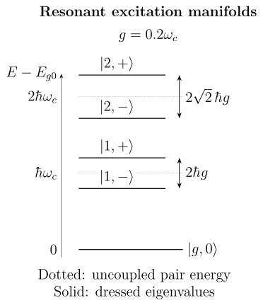
At atom–cavity resonance, the interaction couples $|e,N-1\rangle$ and $|g,N\rangle$ within each fixed-excitation manifold. Their symmetric and antisymmetric combinations form a doublet separated by $2\hbar g\sqrt N$. The vacuum state $|g,0\rangle$ remains unpaired.

Bare character across a cavity resonance

As $\Delta_c$ is swept through zero, every $N\ge1$ manifold has an avoided crossing. Its minimum gap is

$$\Delta E_N^{\min} = 2\hbar g\sqrt N.$$

The bare content changes with detuning:

$$|\langle e,N-1|N,+\rangle|^2 = \frac12 \left( 1+\frac{\Delta_c}{\Omega_N} \right).$$

Thus the same spectral curve contains both a coupling measurement and a state-composition map. Measuring only the separation does not by itself determine which bare component a branch contains; the sign of detuning and the branch convention are also required.

Entanglement in Quantized Dressed States

For a physical quantized mode, the resonant state

$$|N,+\rangle = \frac1{\sqrt2} \left( |e,N-1\rangle + |g,N\rangle \right)$$

is not an atomic superposition multiplied by a field state. The two photon states are orthogonal, so the atom and mode are entangled.

Tracing over the field gives

$$\rho_{\mathrm{atom}}^{(N,+)} = \cos^2\frac{\theta_N}{2} |e\rangle\langle e| + \sin^2\frac{\theta_N}{2} |g\rangle\langle g|.$$

There is no off-diagonal atomic coherence in this reduced state, even though the joint state is pure. The entanglement entropy is

$$S_N = - p_N\ln p_N - (1-p_N)\ln(1-p_N),$$

where

$$p_N = \cos^2\frac{\theta_N}{2}.$$

At resonance, $p_N=1/2$ and $S_N=\ln2$. Far from resonance, one component dominates and the entropy tends to zero.

This is a sharp difference from a semiclassical dressed state

$$c_e|e\rangle+c_g|g\rangle,$$

which is a pure state of the atom because the classical source is not part of the Hilbert space. Replacing a quantized field by a classical amplitude can therefore reproduce mean coherent dynamics while discarding atom–field entanglement.

Semiclassical Limit of a Quantized Mode

Let the mode begin in a coherent state $|\alpha\rangle$ with

$$\bar n = |\alpha|^2.$$

The Jaynes–Cummings interaction samples many excitation manifolds. Near the center of a large photon-number distribution,

$$2g\sqrt N \simeq 2g\sqrt{\bar n},$$

so the corresponding classical Rabi-frequency coefficient is

$$\Omega \simeq 2g|\alpha|.$$

This is a local, large-occupation correspondence, not an operator identity. A coherent state has photon-number variance

$$\operatorname{Var}(n) = \bar n,$$

and therefore contains a spread of Rabi frequencies: $2g\sqrt{n+1}$ for an initially excited atom and $2g\sqrt n$ for an initially ground-state atom. At short times and large $\bar n$, the fractional spread is small and a classical drive is accurate. At longer times, the components dephase and can later rephase, producing collapse and revival of the inversion. That photon-number-resolved behavior is absent from a deterministic single-frequency classical field.

The precise large-field limit must also specify what is held fixed. Taking $|\alpha|\to\infty$ at fixed $g$ makes the drive diverge. A controlled semiclassical scaling keeps $g|\alpha|$ finite while suppressing relative field fluctuations.

Floquet and Dressed-State Dictionary

For a classical periodic Hamiltonian,

$$H(t+T) = H(t), \qquad T = \frac{2\pi}{\omega_L},$$

Floquet states have the form

$$\begin{gathered} |\psi_\alpha(t)\rangle = e^{-i\varepsilon_\alpha t/\hbar} |u_\alpha(t)\rangle, \\ |u_\alpha(t+T)\rangle = |u_\alpha(t)\rangle. \end{gathered}$$

The quasienergy is defined modulo $\hbar\omega_L$:

$$\varepsilon_\alpha \sim \varepsilon_\alpha+m\hbar\omega_L, \qquad m\in\mathbb Z.$$

Expanding $|u_\alpha(t)\rangle$ in Fourier harmonics produces an extended matrix with repeated bare levels shifted by $m\hbar\omega_L$. Near a one-photon resonance, retaining the nearly degenerate pair gives the same $2\times2$ RWA matrix that defines the semiclassical dressed states.

This establishes a useful dictionary:

Quantized single mode	Classical Floquet drive
$\lvert g,n\rangle$, $\lvert e,n-1\rangle$	bare state with Fourier index
physical photon occupation	harmonic bookkeeping index
joint energy eigenvalue	quasienergy modulo $\hbar\omega_L$
atom–field entanglement possible	no source subsystem in the model
number fluctuations are physical	drive amplitude prescribed

The analogy is strongest for a highly occupied, nearly monochromatic mode and near-resonant dynamics over times for which back-action and photon-number dispersion are negligible.

Outside the RWA, a Floquet calculation can retain many harmonics and reveal multiphoton avoided crossings and the Bloch–Siegert shift. A fully quantized Rabi model can retain counter-rotating terms. These extensions are again related, but their state spaces and observables should not be conflated.

How Dressed States Become Observable

Eigenvectors are not observed directly. A measurement accesses transition frequencies, line strengths, time evolution, or correlations.

Weak-probe spectroscopy

Suppose the control does not dress a third state $|r\rangle$, and a weak probe couples it only to the bare state $|e\rangle$. If

$$\langle r|D|g\rangle = 0, \qquad \langle r|D|e\rangle = d_{re},$$

then the dressed-state matrix elements are

$$\begin{aligned} \langle r|D|+\rangle &= d_{re} \cos\frac{\theta}{2}, \\ \langle r|D|-\rangle &= - d_{re} \sin\frac{\theta}{2}. \end{aligned}$$

The squared dipole matrix elements therefore have the ratio

$$S_+ : S_- = \cos^2\frac{\theta}{2} : \sin^2\frac{\theta}{2}.$$

These give relative integrated absorption strengths from a common populated $|r\rangle$ when other frequency prefactors are effectively equal. For emission from the dressed branches, their populations also enter. Peak heights further depend on linewidths. At resonance the two dipole strengths are equal; far away one vanishes.

The observed peaks are separated by dressed energy differences only when the relevant linewidths, probe back-action, populations, and interference paths are included consistently. For the full three-level spectrum, see Autler–Townes Splitting.

Time-domain interference

If a bare state is prepared suddenly, the two dressed components acquire a relative phase

$$\Delta\varphi(t) = \frac{ \varepsilon_+-\varepsilon_- }{ \hbar } t = \Omega_Rt.$$

Bare-state population oscillations are an interferometric measurement of that phase. The frequency reveals the dressed gap, while the oscillation contrast reveals the mixing angle and state preparation.

Emission and dressed-state transitions

Spontaneous emission acts through an operator such as $\sigma_-$. Written in the dressed basis, this operator has several matrix elements between neighboring atom–photon manifolds. Consequently, a strongly driven two-level emitter can radiate at more than one dressed transition frequency. In the resonant, well-resolved regime this underlies the Mollow triplet.

The radiative reservoir, linewidths, and fluorescence spectrum are not contained in the Hermitian two-state eigenproblem alone. They require the open-system treatment developed in Spontaneous Emission and Optical Bloch Equations.

Cavity QED Connection

In cavity QED, the quantized dressed doublets can be spectroscopically resolved because the atom repeatedly exchanges an excitation with a long-lived resonator mode. In the one-excitation sector, a useful non-Hermitian pole model is

$$\frac{H_{\mathrm{eff}}}{\hbar} = \begin{pmatrix} \omega_0-i\gamma/2 & g \\ g & \omega_c-i\kappa/2 \end{pmatrix},$$

where $\gamma$ is the atomic population-decay rate into noncavity channels and $\kappa$ is the cavity energy-decay rate in this convention. Pure dephasing is absent; the atomic optical coherence therefore decays at $\gamma/2$. The complex poles are

$$\widetilde\omega_\pm = \frac{\omega_0+\omega_c}{2} - i\frac{\gamma+\kappa}{4} \pm \sqrt{ g^2 + \frac14 \left[ \Delta_c - i\frac{\gamma-\kappa}{2} \right]^2 }.$$

The real parts give pole frequencies and the imaginary parts give amplitude decay rates; measured spectral maxima need not coincide with the real parts. At exact resonance, the square root has a nonzero real part when

$$g > \frac{|\kappa-\gamma|}{4}.$$

That algebraic pole-splitting condition is not, by itself, a universal criterion for visibly resolving two peaks. Resolvability depends on the combined widths, drive and detection port, background, and fitting model. Likewise, the cooperativity

$$C = \frac{4g^2}{\kappa\gamma}$$

tests coherent coupling against dissipation but answers a different question from peak separation.

The same linear two-mode equations can describe coupled classical oscillators. A weak-excitation doublet alone therefore does not establish field quantization (Zhu and colleagues). Resolving the excitation-dependent Jaynes–Cummings ladder probes its anharmonicity (Fink and colleagues); nonclassical correlations provide complementary information.

The closed dressed-state spectrum explains the underlying level structure. Cavity QED develops the mode overlap, linewidth conventions, dissipative spectrum, Purcell limit, and measured transmission or reflection. The open-system cavity-QED map continues to conditional output records and trajectories.

Beyond the Ideal Two-State RWA

Counter-rotating terms

The quantum Rabi Hamiltonian contains

$$\hbar g \left( a+a^\dagger \right) \left( \sigma_++\sigma_- \right).$$

Besides the Jaynes–Cummings exchange terms, it includes

$$a\sigma_- \qquad\text{and}\qquad a^\dagger\sigma_+.$$

These terms do not conserve $\mathcal N$. The independent two-dimensional manifolds disappear; the discrete parity $\sigma_z(-1)^{a^\dagger a}$ remains conserved in the ideal Rabi model. Perturbatively they produce shifts such as the Bloch–Siegert correction. In ultrastrong coupling, the exact eigenstates contain contributions from many bare excitation sectors and the phrase “one photon in the dressed ground state” becomes measurement-model dependent.

Multilevel matter

A real atom or molecule may have several nearby states coupled by the same field. Then the dressed Hamiltonian is larger than $2\times2$, and dark states, multiple avoided crossings, tensor light shifts, and leakage can appear. The two-state mixing angle remains useful only after the neglected levels have been shown to be perturbative, or exactly decoupled by a symmetry or selection rule.

Near-degenerate magnetic or hyperfine manifolds are especially sensitive to polarization and selection rules. A measured splitting cannot be assigned to one $\Omega$ until the complete coupled subspace has been checked.

Spatial and motional dependence

If the coupling varies with position,

$$\Omega = \Omega(\mathbf r),$$

then the dressed energies define position-dependent adiabatic potentials. Atomic motion can also drive transitions between local dressed branches. The relevant small parameter compares motional matrix elements of the position-dependent basis to the local dressed gap. Treating $\varepsilon_\pm(\mathbf r)$ as ordinary scalar potentials without those derivative couplings can fail near nodes and avoided crossings. Even in a single adiabatic branch, projected kinetic energy generally contributes a geometric vector potential and a scalar correction, in addition to the local eigenvalue.

Dissipation and noise

Hermitian dressed eigenstates are not generally eigenmodes of a Lindblad generator. Relaxation, dephasing, drive noise, and cavity loss change the steady state and broaden transitions. In weak dissipation, the Hamiltonian dressed basis is often a useful starting point for a secular master equation. Near degeneracies or for structured reservoirs, secularizing in that basis may erase important interference.

The phrase “dressed-state lifetime” must therefore identify:

• the prepared branch;
• the decay and dephasing channels;
• whether the quoted quantity is a population lifetime, coherence time, or spectral linewidth;
• the approximation used to transform the bath coupling operators.

Exercises

1. A phase cycle and geometric phase

Keep $\theta$ fixed with a nonzero gap and vary $\phi$ adiabatically from 0 to $2\pi$. Find the geometric phase of $|+\rangle$ in the eigenvector convention above. Why can a time-dependent drive phase matter even though the instantaneous eigenvalues do not depend on it?

Solution

The chosen vector is periodic in $\phi$ and

$$i\langle+|\partial_\phi+\rangle=-\sin^2(\theta/2), \qquad \gamma_+=-\pi(1-\cos\theta)\pmod{2\pi}.$$

It is minus half the solid angle traced by the effective-field direction. The lower branch gives the opposite phase modulo $2\pi$. A phase variation rotates eigenvectors, producing geometric phase during adiabatic motion and potentially transitions otherwise. It cannot be treated as a sequence of unrelated static rephasings without their time-derivative term.

2. Recover Rabi oscillations from dressed phases

Take $\phi=0$ and prepare $|g\rangle$ suddenly at $t=0$. Use the dressed basis to find the excited-state probability for constant $\Omega$ and $\Delta$.

Solution

The inverse transformation gives

$$|g\rangle = \sin\frac{\theta}{2}|+\rangle + \cos\frac{\theta}{2}|-\rangle.$$

After time $t$,

$$|\psi(t)\rangle = \sin\frac{\theta}{2} e^{-i\Omega_Rt/2} |+\rangle + \cos\frac{\theta}{2} e^{+i\Omega_Rt/2} |-\rangle.$$

Projecting onto $|e\rangle$ gives

$$\begin{aligned} c_e(t) &= - 2i \sin\frac{\theta}{2} \cos\frac{\theta}{2} \sin\frac{\Omega_Rt}{2} \\ &= - i\sin\theta \sin\frac{\Omega_Rt}{2}. \end{aligned}$$

Therefore

$$P_e(t) = \frac{\Omega^2}{\Omega_R^2} \sin^2 \left( \frac{\Omega_Rt}{2} \right).$$

The oscillation is interference between stationary dressed components. Detuning increases the phase-evolution frequency but reduces the mixing factor $\Omega^2/\Omega_R^2$.

3. Track branch identity across resonance

For fixed $\Omega>0$, determine the limiting bare character of $|+\rangle$ and $|-\rangle$ as $\Delta\to+\infty$ and $\Delta\to-\infty$. Explain why “the excited dressed state” is an unsafe global label.

Solution

When $\Delta\to+\infty$,

$$\theta\to0,$$

so

$$|+\rangle\to|e\rangle, \qquad |-\rangle\to e^{i\phi}|g\rangle.$$

When $\Delta\to-\infty$,

$$\theta\to\pi,$$

so

$$|+\rangle\to e^{i\phi}|g\rangle, \qquad |-\rangle\to-|e\rangle.$$

The upper and lower eigenvalue branches are continuous, but each exchanges its bare identity through the avoided crossing. A label based on bare character must therefore include the side of resonance or an explicit adiabatic path.

4. Adiabaticity of a detuning sweep

Let $\Omega$ be constant and sweep

$$\Delta(t) = vt.$$

Find $|\dot\theta|$, locate its maximum, and obtain a simple local adiabaticity condition. For

$$\begin{gathered} \dfrac{\Omega}{2\pi} = 100\ \mathrm{kHz}, \\ \dfrac{|v|}{2\pi} = 1.0\times10^{10}\ \mathrm{Hz\,s^{-1}}, \end{gathered}$$

estimate the Landau–Zener diabatic probability. Convert all quantities consistently to angular units.

Solution

For constant $\Omega$,

$$|\dot\theta| = \frac{ \Omega|v| }{ \Delta^2+\Omega^2 }.$$

It is largest at resonance:

$$|\dot\theta|_{\max} = \frac{|v|}{\Omega}.$$

Comparing this with the minimum gap frequency $\Omega$ gives

$$|v| \ll \Omega^2.$$

Numerically,

$$\Omega = 2\pi\times10^5\ \mathrm{s^{-1}},$$

and

$$|v| = 2\pi\times10^{10}\ \mathrm{s^{-2}}.$$

The exponent is

$$\begin{aligned} \frac{\pi\Omega^2}{2|v|} &= \frac{ \pi(2\pi\times10^5)^2 }{ 2(2\pi\times10^{10}) } \\ &= \pi^2 \simeq 9.87. \end{aligned}$$

Thus

$$P_{\mathrm{diab}} \simeq e^{-9.87} \simeq 5.2\times10^{-5}.$$

The transfer is highly, though not perfectly, adiabatic in the ideal infinite-sweep model.

5. The detected channel selects different lines

At resonance choose $|N,s\rangle=(|e,N-1\rangle+s|g,N\rangle)/\sqrt2$, where $s=\pm1$. For $N\ge2$, calculate transitions to $|N-1,t\rangle$ through atomic emission $\sigma_-$ and through cavity leakage $a$. Compare their relative strengths for large $N$.

Solution

Apply the lowering operator before taking the final overlap:

$$\begin{aligned} \langle N-1,t|\sigma_-|N,s\rangle&=t/2,\\ \langle N-1,t|a|N,s\rangle&= \frac{\sqrt{N-1}+st\sqrt N}{2}. \end{aligned}$$

All four atomic-channel matrix elements have squared magnitude $1/4$. For cavity leakage, same-branch strengths approach $N$, whereas opposite-branch strengths approach $1/(16N)$. The ratio is therefore about $16N^2$. Actual intensities also require initial populations and the channel’s coupling to the detector. The $N=1$ transition ends in the unpaired vacuum state and must be calculated separately.

6. Entanglement away from resonance

For the state $|N,+\rangle$, compute the atomic purity

$$\mathcal P = \operatorname{Tr} \left[ \left( \rho_{\mathrm{atom}}^{(N,+)} \right)^2 \right].$$

Evaluate it on resonance and in the limit $|\Delta_c|\gg g\sqrt N$.

Solution

The reduced atomic probabilities are

$$p = \cos^2\frac{\theta_N}{2}, \qquad 1-p = \sin^2\frac{\theta_N}{2}.$$

Hence

$$\mathcal P = p^2+(1-p)^2.$$

Using

$$2p-1 = \cos\theta_N = \frac{\Delta_c}{\Omega_N},$$

one finds

$$\mathcal P = \frac12 \left[ 1+ \frac{\Delta_c^2}{\Omega_N^2} \right].$$

At resonance,

$$\mathcal P = \frac12,$$

the minimum purity for a two-level reduced state, corresponding to maximal atom–mode entanglement in this two-term Schmidt decomposition.

For $|\Delta_c|\gg g\sqrt N$,

$$\frac{\Delta_c^2}{\Omega_N^2} \to 1,$$

so $\mathcal P\to1$. The dressed state approaches a bare product state.

7. Predict weak-probe line strengths

Prepare atoms in a third state $|r\rangle$ that couples only to $|e\rangle$. Find the relative squared dipole matrix elements for absorption to $|+\rangle$ and $|-\rangle$ for

$$\Delta = \frac34\Omega_R.$$

What additional information is needed before claiming that two peaks will be visible?

Solution

The condition gives

$$\cos\theta = \frac34.$$

Therefore

$$\cos^2\frac{\theta}{2} = \frac{1+\cos\theta}{2} = \frac78,$$

and

$$\sin^2\frac{\theta}{2} = \frac18.$$

For these dipole strengths,

$$S_+:S_- = 7:1.$$

Two eigenvalues do not guarantee two visible peaks. One must also know the dressed separation, homogeneous and inhomogeneous linewidths, dressed-state populations, probe strength, competing matrix elements, interference paths, instrument response, and signal-to-noise ratio.

8. Separate Floquet harmonics from photons

Consider a two-level atom driven by a prescribed classical periodic field. A Floquet calculation labels basis vectors by an integer $m$. Decide which of the following statements are valid, and justify each answer:

1. measuring the cavity photon number measures $m$;
2. quasienergies differing by $\hbar\omega_L$ represent equivalent Floquet zones;
3. a Floquet state necessarily entangles the atom with the source;
4. a highly occupied coherent quantized mode can approximate the semiclassical Rabi coefficient.

Solution

1. Invalid. A prescribed classical drive has no cavity Hilbert space or photon-number operator. The integer $m$ labels a Fourier harmonic in extended Floquet space.
2. Valid. Multiplying the periodic part by $e^{im\omega_Lt}$ shifts the quasienergy by $m\hbar\omega_L$ without changing the physical solution.
3. Invalid. The classical source is not a subsystem of the model, so atom–source entanglement is undefined there. The atomic state may still be a coherent superposition.
4. Valid with qualifications. For a coherent state with large $\bar n$, the matrix element near the distribution center gives $\Omega\simeq2g\sqrt{\bar n}=2g|\alpha|$. The approximation is limited by photon-number dispersion, back-action, and the timescale of interest.

References

• S. H. Autler and C. H. Townes, “Stark effect in rapidly varying fields,” Physical Review 100, 703–722 (1955).
• A. Blais, A. L. Grimsmo, S. M. Girvin, and A. Wallraff, “Circuit quantum electrodynamics,” Reviews of Modern Physics 93, 025005 (2021).
• C. Cohen-Tannoudji, “Manipulating atoms with photons,” Reviews of Modern Physics 70, 707–719 (1998).
• C. Cohen-Tannoudji, J. Dupont-Roc, and G. Grynberg, Atom–Photon Interactions: Basic Processes and Applications (Wiley, 1992), especially Chapters IV and VI.
• J. M. Fink, M. Göppl, M. Baur, R. Bianchetti, P. J. Leek, A. Blais, and A. Wallraff, “Climbing the Jaynes–Cummings ladder and observing its nonlinearity in a cavity QED system,” Nature 454, 315–318 (2008).
• S. Haroche and J.-M. Raimond, Exploring the Quantum: Atoms, Cavities, and Photons (Oxford University Press, 2006).
• E. T. Jaynes and F. W. Cummings, “Comparison of quantum and semiclassical radiation theories with application to the beam maser,” Proceedings of the IEEE 51, 89–109 (1963).
• B. R. Mollow, “Power spectrum of light scattered by two-level systems,” Physical Review 188, 1969–1975 (1969).
• H. Sambe, “Steady states and quasienergies of a quantum-mechanical system in an oscillating field,” Physical Review A 7, 2203–2213 (1973).
• J. H. Shirley, “Solution of the Schrödinger equation with a Hamiltonian periodic in time,” Physical Review 138, B979–B987 (1965).
• B. W. Shore and P. L. Knight, “The Jaynes–Cummings model,” Journal of Modern Optics 40, 1195–1238 (1993).
• Y. Zhu, D. J. Gauthier, S. E. Morin, Q. Wu, H. J. Carmichael, and T. W. Mossberg, “Vacuum Rabi splitting as a feature of linear-dispersion theory: Analysis and experimental observations,” Physical Review Letters 64, 2499–2502 (1990).