Mutual Information in Many-Body Systems

Quantum mutual information measures the total correlation between two declared parts of a many-body state. Let the full system be divided into disjoint regions

$$\Omega = A\sqcup B\sqcup C,$$

where $C$ may be empty. Starting from a state $\rho_\Omega$, form

$$\rho_{AB} = \operatorname{Tr}_C\rho_\Omega.$$

The mutual information is

$$I(A:B)_\rho := S(\rho_A) + S(\rho_B) - S(\rho_{AB}).$$

This combination answers a sharper question than either regional entropy alone:

How much of the uncertainty in $A$ and $B$ is shared rather than independent?

In a mixed thermal state, $S(\rho_A)$ and $S(\rho_B)$ can both be extensive even when the state has no correlations at all. Their independent bulk contributions cancel in $I(A:B)$. In a pure state split into complementary regions, by contrast, the mutual information is twice the entanglement entropy. Between separated regions it probes all correlation channels at once, including classical, quantum, symmetry-sector, constraint-induced, and long-range contributions.

That breadth is both the strength and the main caution. Nonzero mutual information does not by itself prove entanglement, identify a phase, locate a critical point, or reveal which observables carry the correlation.

Helpful background. Mutual information supplies the finite-system definition and relative-entropy identity; connected correlation functions explains the operator correlations bounded below.

Regional states and spatial geometry

State and regions

Unless stated otherwise:

• $\rho_\Omega$ is a normalized state on a finite lattice Hilbert space;
• $A$ and $B$ are disjoint sets of sites, orbitals, modes, or local degrees of freedom;
• $C=\Omega\setminus(A\cup B)$ is the environment traced out before evaluating $I(A:B)$;
• $S(\rho)=-\operatorname{Tr}(\rho\ln\rho)$ uses natural logarithms, so information is measured in nats;
• continuum and gauge-theory statements require additional regulator and algebra choices.

The subsystem choice is physical data. A spatial region, a momentum-space block, an orbital set, and a particle partition generally produce different reduced states and different mutual informations.

Three geometries

The same formula appears in three geometrically distinct settings.

Geometry	Environment $C$	Typical question
complementary cut $B=\bar A$	empty	how much total correlation crosses one cut?
adjacent $A$ and $B$ inside $\Omega$	nonempty or empty	how much correlation is localized near their shared interface?
separated $A$ and $B$	nonempty buffer	how does total correlation decay with separation?

These geometries should not be compared without matching sizes, boundaries, separation, total volume, and state preparation.

Logarithm base

Changing the logarithm base rescales every entropy and mutual information by the same constant. With base $2$,

$$I_{\mathrm{bits}}(A:B) = \frac{I(A:B)}{\ln2}$$

is measured in bits. The descriptive subscript distinguishes this base change from a second Rényi mutual information; a superscript such as $I^{(2)}$ is reserved for Rényi constructions.

Core Identities for Many-Body Use

Relative entropy to the product state

The central identity is

$$I(A:B)_\rho = D\!\left( \rho_{AB} \middle\| \rho_A\otimes\rho_B \right),$$

where $D(\rho\|\sigma)$ is quantum relative entropy. Therefore

$$I(A:B)_\rho \ge 0,$$

with equality exactly when

$$\rho_{AB} = \rho_A\otimes\rho_B.$$

The comparison product uses the actual marginals of the state. Mutual information removes local mixedness while retaining every deviation of the joint state from independence.

Upper bounds

The Araki–Lieb inequality gives

$$I(A:B) \le 2\min\{S_A,S_B\}.$$

For finite local Hilbert spaces,

$$I(A:B) \le 2\ln\min\{d_A,d_B\}.$$

These are dimension bounds, not expected scaling laws. A much smaller value can follow from locality, temperature, separation, symmetry, or the state class.

Data processing

Local quantum channels cannot increase mutual information. If $\Phi_A$ and $\Phi_B$ act independently,

$$I(A':B')_{(\Phi_A\otimes\Phi_B)(\rho)} \le I(A:B)_\rho.$$

In particular, discarding degrees of freedom cannot reveal more total correlation:

$$\begin{aligned} A&\subseteq A', &B&\subseteq B', \\ I(A:B)&\le I(A':B'). \end{aligned}$$

This monotonicity is useful when comparing single sites, small blocks, and enlarged blocks. It also explains why coarse local measurements provide lower bounds rather than exact reconstructions of the quantum mutual information.

Local-unitary invariance

Independent unitary changes of basis inside the regions preserve the value:

$$I(A:B)_{(U_A\otimes U_B)\rho(U_A^\dagger\otimes U_B^\dagger)} = I(A:B)_\rho.$$

An orbital or mode transformation that mixes $A$ with $B$ changes the partition and need not preserve it.

Pure-State Geometry

Complementary regions

If the global state on $AB$ is pure,

$$S_{AB}=0, \qquad S_A=S_B,$$

and hence

$$I(A:B) = 2S_A.$$

For a complementary pure-state cut, mutual information contains no independent information beyond the entanglement entropy. The factor of two matters: a single Bell pair crossing the cut contributes $\ln2$ to $S_A$ and $2\ln2$ to $I(A:B)$.

Embedded regions of a pure state

Now let $ABC$ be pure and trace out a nonempty $C$. Then

$$S_{AB}=S_C,$$

so

$$I(A:B) = S_A+S_B-S_C.$$

This is generally smaller than $2\min\{S_A,S_B\}$. Correlations that either region shares with $C$ do not automatically become correlations between $A$ and $B$.

The distinction is crucial for spatial studies. Two disjoint intervals in a pure chain have a mixed joint state because the sites between and outside them were traced out.

A Bell-pair boundary count

Suppose the global state is a product of local states and $n_\partial$ Bell pairs, each crossing a complementary spatial cut. Then

$$S_A = n_\partial\ln2,$$

and

$$I(A:\bar A) = 2n_\partial\ln2.$$

The mutual information therefore obeys the same boundary count, with twice the pure-state entropy coefficient. This fixed-point example motivates an area law but does not prove one for generic interacting states.

Reading Spatial Mutual Information

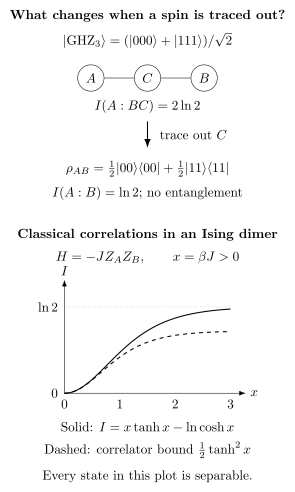
Two exact examples distinguish total correlation from entanglement. In the three-spin GHZ state, $I(A:BC)=2\ln2$; after tracing out $C$, the remaining two-spin state is a separable classical mixture with $I(A:B)=\ln2$. The lower plot shows the separable Ising-dimer Gibbs state: its mutual information approaches one classical bit, while the connected $Z$ correlator gives the lower bound $I\ge\tfrac12\tanh^2x$, with $x=\beta J$.

Adjacent regions

When $A$ and $B$ share a boundary, short-distance degrees of freedom can correlate strongly across that interface. In a short-range thermal state, the leading volume entropy cancels, leaving an interface-controlled contribution under suitable assumptions.

On a lattice the result is finite. In a continuum theory with a sharp shared boundary, the individual entropies and their combination can retain ultraviolet sensitivity. Adjacency should not be confused with the regulator-independent separated-region construction.

Separated regions

Let $r$ denote the minimum distance between $A$ and $B$. For separated regions, the buffer $C$ removes a shared ultraviolet boundary. In many gapped ground states and noncritical thermal states, $I(A:B)$ decreases rapidly when

$$r \gg \xi,$$

where $\xi$ is an appropriate correlation length. The precise upper bound and decay law require assumptions about locality, the state family, region sizes, and sometimes the phase.

At criticality, scale invariance can replace exponential decay by a power-law or cross-ratio dependence. The functional form is theory and geometry dependent; a generic power law should not be assigned a universal exponent without specifying the operator content and limiting regime.

Region size matters

Two single-site regions may have weak mutual information while two larger blocks at the same separation have a substantial value because many weak channels accumulate. Report at least

$$|A|, \qquad |B|, \qquad r, \qquad L,$$

along with boundary conditions and shape.

Mutual Information and Connected Correlators

A rigorous lower bound

Let $O_A$ and $O_B$ be bounded operators supported in $A$ and $B$. Define the connected correlator

$$C_{AB}(O_A,O_B) := \langle O_AO_B\rangle - \langle O_A\rangle \langle O_B\rangle.$$

Because

$$C_{AB} = \operatorname{Tr} \left[ \left( \rho_{AB}-\rho_A\otimes\rho_B \right) O_A\otimes O_B \right],$$

trace-norm duality gives

$$|C_{AB}| \le \left\| \rho_{AB}-\rho_A\otimes\rho_B \right\|_1 \|O_A\|\,\|O_B\|.$$

Quantum Pinsker inequality in nats states

$$I(A:B) \ge \frac12 \left\| \rho_{AB}-\rho_A\otimes\rho_B \right\|_1^2.$$

Combining the two yields

$$I(A:B) \ge \frac{ |C_{AB}(O_A,O_B)|^2 }{ 2\|O_A\|^2\|O_B\|^2 }.$$

Thus any nonzero bounded connected correlator proves nonzero mutual information. Conversely, sufficiently small mutual information forces every bounded connected correlator between the two regions to be small.

The converse does not follow from a short operator list

Suppose numerical data show

$$C_{AB}(O_A^{(k)},O_B^{(k)}) \approx 0$$

for several selected pairs. This does not prove $I(A:B)\approx0$. The reduced state may contain:

• higher-order correlations;
• correlations in an unmeasured symmetry channel;
• string or loop correlations;
• a shared conserved-sector label;
• correlations distributed over many individually weak operators.

Full mutual information summarizes the entire $\rho_{AB}$, whereas a correlator probes one direction in operator space.

Long-range order

If normalized bounded order-parameter operators retain

$$\lim_{r\to\infty} |C_{AB}(r)| > 0,$$

the lower bound prevents $I(A:B)$ from vanishing at large separation. The reverse statement needs care: nonvanishing mutual information may come from a global constraint, a finite-volume cat state, or another channel rather than the proposed order parameter.

Thermal States

Infinite temperature

For an unconstrained lattice with local Hilbert-space dimensions $d_A$ and $d_B$, the infinite-temperature state factorizes:

$$\rho_0 = \frac{I_A}{d_A} \otimes \frac{I_B}{d_B}.$$

Although

$$S_A=\ln d_A, \qquad S_B=\ln d_B,$$

the joint entropy is their sum, and

$$I(A:B)=0.$$

This is the cleanest demonstration that extensive local entropy is not correlation and not entanglement.

Cancellation of the bulk thermal term

In a regular homogeneous thermal phase, suppose

$$\begin{aligned} S_A &= s_{\mathrm{th}}V_A+\delta_A, \\ S_B &= s_{\mathrm{th}}V_B+\delta_B, \\ S_{AB} &= s_{\mathrm{th}}(V_A+V_B)+\delta_{AB}. \end{aligned}$$

Then

$$I(A:B) = \delta_A+\delta_B-\delta_{AB}.$$

The volume term cancels exactly. The remainder may contain interface, corner, finite-size, conservation-law, critical, or long-range-interaction contributions.

The cancellation is algebraic, but extracting the small remainder numerically can be difficult because it subtracts three much larger quantities.

Gibbs-state area bound

Take $A$ and $B$ to be complementary parts of a finite tensor-product Hilbert space, and let

$$\rho_{AB} = \frac{e^{-\beta H}}{Z},\qquad \beta>0,$$

where the trace defining $Z$ runs over that full space. Use a local decomposition

$$H = H_A+H_B+H_\partial,$$

where $H_\partial$ contains interactions crossing the cut. The product $\rho_A\otimes\rho_B$ has the same expectations of $H_A$ and $H_B$ as $\rho_{AB}$.

The product trial state is admissible in this unconstrained Gibbs problem. Positivity of $D(\rho_A\otimes\rho_B\|\rho_{AB})$ gives the bound directly:

$$D(\rho_A\otimes\rho_B\|\rho_{AB}) ={}\beta\operatorname{Tr}[H_\partial(\rho_A\otimes\rho_B-\rho_{AB})] -I(A:B)\ge0.$$

Consequently,

$$I(A:B) \le \beta \operatorname{Tr} \left[ H_\partial \left( \rho_A\otimes\rho_B-\rho_{AB} \right) \right].$$

Using the operator norm,

$$I(A:B) \le 2\beta\|H_\partial\|.$$

For bounded finite-range interactions with

$$\|H_\partial\| \le J|\partial_E A|,$$

one obtains

$$I(A:B) \le 2\beta J|\partial_E A|.$$

This is a thermal area-law upper bound. It can be loose, especially as $\beta$ grows. Projection onto a fixed total charge changes the hypothesis: the product of the marginals may leave that sector, so this trial-state argument no longer applies. The one-particle example below has positive mutual information even for $H=0$ restricted to its fixed-number sector.

For embedded or separated $A,B$ in a larger Gibbs system $\Omega$, $\rho_{AB}$ is generally not a Gibbs state of $H_A+H_B$ plus their direct interface. Instead data processing gives $I(A:B)\le I(A:\Omega\setminus A)$, to which the full Gibbs boundary bound applies. Area laws explains the boundary conventions.

Exact Ising-dimer example

Consider two spins with

$$H = -J\sigma_1^z\sigma_2^z, \qquad x:=\beta J,\qquad J>0,\quad\beta>0.$$

The Gibbs state is diagonal and separable. Both one-spin marginals are maximally mixed, while the joint probabilities favor aligned outcomes. Its mutual information is

$$I(1:2) = x\tanh x - \ln\cosh x.$$

At high temperature,

$$I(1:2) = \frac{x^2}{2} - \frac{x^4}{4} + O(x^6).$$

At zero temperature approached through the Gibbs state,

$$I(1:2) \longrightarrow \ln2.$$

The limiting state is the classical mixture of the two aligned configurations. The nonzero result is one shared classical bit, not entanglement.

Thermal entanglement is a separate question

An interacting Gibbs state can be entangled at nonzero temperature. Mutual information then combines the quantum contribution with all classical and thermal correlations. To isolate entanglement, use a measure or witness appropriate to the bipartition, such as negativity and the PPT criterion where applicable.

The implication is one-way:

$$I(A:B)=0 \quad\Longrightarrow\quad \text{no entanglement},$$

but

$$I(A:B)>0$$

does not distinguish separable from entangled states.

Constraints and Ensembles

Fixed charges create correlations

The phrase “infinite temperature” is incomplete without the ensemble. The maximally mixed state on the full tensor-product Hilbert space factorizes. The maximally mixed state inside a fixed total-charge sector generally does not.

Consider one particle uniformly mixed over $L$ sites:

$$\rho^{(1)} = \frac1L \sum_{j=1}^{L} \lvert j\rangle\langle j\rvert.$$

Partition the lattice into $L_A=fL$ and $L_B=(1-f)L$ sites. Region $A$ is either empty or contains the particle. Its entropy is

$$S_A = H_2(f) + f\ln L_A,$$

where

$$H_2(f) := -f\ln f -(1-f)\ln(1-f).$$

Similarly,

$$S_B = H_2(f) + (1-f)\ln L_B,$$

while

$$S_{AB}=\ln L.$$

The mutual information is therefore

$$I(A:B) = H_2(f).$$

At $f=1/2$, the fixed-number constraint contributes $\ln2$. This is not an interaction-generated correlation; it is the shared information that if the particle is in one region it is absent from the other.

Canonical versus grand-canonical comparisons

At finite size, global conservation can produce constant, logarithmic, or other subextensive contributions absent from an unconstrained ensemble. A reliable comparison records:

• whether total charge, magnetization, momentum, or parity is fixed;
• whether the reduced state retains block labels;
• whether the same ensemble is used at every size;
• which limit is taken before the subsystem fraction is fixed.

Ensemble Equivalence explains when local thermodynamic predictions converge and why information measures can remain sensitive to global constraints at finite size.

Ordered, Critical, and Topological Regimes

Finite-volume cat states

For the $N$-spin GHZ state

$$\lvert\mathrm{GHZ}_N\rangle = \frac{ \lvert0\rangle^{\otimes N} + \lvert1\rangle^{\otimes N} }{\sqrt2},$$

every nonempty proper region has entropy $\ln2$. If nonempty disjoint $A$ and $B$ do not cover the whole system,

$$S_A=S_B=S_{AB}=\ln2,$$

and

$$I(A:B)=\ln2.$$

After tracing $C$, the coherence between the two global branches is lost, but the shared branch label remains. For a complementary cut,

$$I(A:\bar A)=2\ln2.$$

This difference is a geometry effect, not a contradiction.

In a symmetry-broken phase, a finite-volume symmetric cat state and a phase-selected thermodynamic state can therefore have different long-distance mutual information. State preparation and order of limits must be declared.

Critical scaling

At a continuous transition, long-distance correlations can make block mutual information scale nonanalytically with region size, separation, temperature, or a conformal cross-ratio. This makes mutual information useful for finite-size scaling.

It does not make the location of a maximum universal. Classical and quantum studies show that peaks, crossings, cusps, and subleading singularities depend on:

• the chosen regions;
• whether von Neumann or Rényi quantities are used;
• boundary and corner geometry;
• subsystem fraction;
• analytic background terms;
• finite-size corrections.

A trustworthy critical analysis uses a scaling ansatz and several sizes. It does not identify a transition from one peak alone. Entanglement and criticality and quantum phase transitions develop the scaling analysis.

Topological phases

Mutual information can enter subtraction schemes that cancel local boundary terms, and separated-region patterns can help reveal nonlocal organization. A single value of $I(A:B)$ is nevertheless not a topological invariant. Classical constraints, symmetry breaking, gauge constraints, and ordinary long-range correlations can all produce nonlocal mutual information.

Topological order explains local indistinguishability, global sectors, loop algebra, anyons, and topological entropy.

Continuum and Gauge-Theory Cautions

Positive separation

For sharply separated continuum regions,

$$\operatorname{dist}(A,B)>0,$$

the local ultraviolet divergences in $S_A$, $S_B$, and $S_{A\cup B}$ cancel under standard assumptions. Mutual information can then define a finite, regulator-independent correlation quantity.

This statement is not automatic when the regions touch. As the separation tends to zero, short-distance correlations can make the mutual information diverge.

Algebra choice

Gauge constraints can obstruct a naive tensor factorization of the physical Hilbert space. Different choices of regional operator algebra, centers, edge modes, or extended Hilbert space can alter entropy assignments. State the algebraic prescription before comparing values.

The dedicated Entanglement in QFT Preview develops these issues without importing continuum formulas into a lattice calculation by analogy alone.

Dynamics and locality

For an initial product state of finite-dimensional sites and bounded finite-range interactions, Lieb–Robinson locality constrains correlations created between fixed finite regions. Operators evolved for time $t$ can be approximated within neighborhoods of radius $v_{\mathrm{LR}}t$. Before these neighborhoods overlap, their expectation values factorize in the initial product state, up to the locality tails.

For regions separated by $r$, the resulting correlation scale involves

$$r-2v_{\mathrm{LR}}t.$$

Controlling a complete operator basis on the finite regions then bounds the reduced-state distance from a product; entropy continuity converts that estimate to a mutual-information bound. The prefactors depend on region size and Hilbert-space dimension. One cannot infer a dimension-independent mutual-information estimate from a few two-point correlators.

Small initial $I(A:B)$ alone is not enough. A remote system may already be entangled with a site next to $A$; a local swap can move that existing correlation into $A$ before a new signal could travel from $B$. For initially correlated states, one must also control correlations between enlarged neighborhoods. The Lieb–Robinson bound states the locality assumptions, while operator entanglement and scrambling distinguishes information spreading from transport.

Numerical and Experimental Extraction

Exact diagonalization

For a state represented explicitly:

1. trace out $C$ to obtain $\rho_{AB}$;
2. trace $B$ and $A$ to obtain $\rho_A$ and $\rho_B$;
3. diagonalize all three reduced operators;
4. compute their entropies with one logarithm convention;
5. form $I(A:B)$ only after checking normalization and positivity.

The Hilbert-space cost grows exponentially with $|A\cup B|$. Exploit exact symmetries without dropping sector probabilities from the entropy.

Matrix-product states and operators

For a pure MPS and one contiguous complementary cut, $I(A:\bar A)=2S_A$ follows from the bond Schmidt values. For disjoint regions or a mixed matrix-product operator, one needs the reduced operator on $A\cup B$ as well as its marginals.

Convergence should be tested against:

• bond dimension;
• discarded weight;
• system size and boundary conditions;
• region size and separation;
• purification or operator-space truncation at finite temperature.

An entropy that appears converged does not guarantee that the smaller difference $I(A:B)$ is converged.

Quantum Monte Carlo and replicas

Replica or swap-operator methods naturally estimate integer-order Rényi entropies. One may form a quantity such as

$$I^{(2)}_{\mathrm{comb}}(A:B) :=S_2(A)+S_2(B) {}-S_2(AB).$$

This is experimentally and numerically useful, but it is not the von Neumann mutual information. For Rényi index $\alpha\ne1$, several inequivalent generalizations exist, and the simple entropy combination need not inherit every property of $I(A:B)$, including the same data-processing and positivity guarantees in full generality.

Report the definition, replica geometry, estimator, and normalization rather than writing an unqualified $I(A:B)$.

For a concrete purity check, take two spins in the diagonal state

$$\rho_{AB}=\operatorname{diag}\!\left(\frac12,\frac14,\frac14,0\right)$$

in the ordered basis $|00\rangle,|01\rangle,|10\rangle,|11\rangle$. Both marginals are $\operatorname{diag}(3/4,1/4)$. Their purities are $5/8$, while the joint purity is $3/8$, giving

$$I^{(2)}_{\mathrm{comb}} =\ln\frac{\operatorname{Tr}\rho_{AB}^2} {\operatorname{Tr}\rho_A^2\,\operatorname{Tr}\rho_B^2} =\ln\frac{24}{25}<0.$$

The same state has positive von Neumann mutual information,

$$I(A:B)=2h_2(1/4)-\frac32\ln2 \simeq0.08495, \qquad h_2(p)=-p\ln p-(1-p)\ln(1-p).$$

It is a separable mixture of product basis states with classical correlations. A negative value of the measured purity combination alone therefore does not diagnose an invalid state or numerical error. Its definition differs from the nonnegative von Neumann quantity.

Two-copy and randomized measurements

Interference between two copies can measure purities and second Rényi entropies. Randomized measurements provide another route to moments of reduced density operators. Both can construct Rényi correlation diagnostics for selected regions.

Experimental claims should report:

• which Rényi index was measured;
• state-preparation and detection errors;
• symmetry or postselection constraints;
• statistical covariance among the three entropy estimates;
• whether the inferred quantity is total correlation or an entanglement witness.

Subtraction error

Suppose estimates obey

$$\widehat S_X = S_X+\varepsilon_X, \qquad X\in\{A,B,AB\}.$$

Then

$$\widehat I-I = \varepsilon_A + \varepsilon_B - \varepsilon_{AB}.$$

If the errors are independent with standard deviations $\sigma_X$,

$$\sigma_I^2 = \sigma_A^2 + \sigma_B^2 + \sigma_{AB}^2.$$

For correlated estimates, the full expression is

$$\sigma_I^2={}\sigma_A^2+\sigma_B^2+\sigma_{AB}^2 +2\operatorname{Cov}(\varepsilon_A,\varepsilon_B) -2\operatorname{Cov}(\varepsilon_A,\varepsilon_{AB}) -2\operatorname{Cov}(\varepsilon_B,\varepsilon_{AB}).$$

Because $I$ may be an area-sized remainder of volume-sized entropies, absolute rather than relative entropy errors control reliability.

Exercises

1. Pure complementary cut

Let $\lvert\Psi\rangle_{AB}$ be pure. Derive $I(A:B)=2S_A$ and evaluate the mutual information for one Bell pair using natural logarithms.

Solution

Purity gives

$$S_{AB}=0$$

and equality of the reduced spectra gives

$$S_A=S_B.$$

Therefore

$$I(A:B) = S_A+S_B-S_{AB} = 2S_A.$$

For one Bell pair,

$$\rho_A=\rho_B=\frac{I}{2},$$

so

$$S_A=S_B=\ln2.$$

Hence

$$I(A:B)=2\ln2.$$

2. Classical Ising dimer

For

$$H=-J\sigma_1^z\sigma_2^z,$$

derive

$$\begin{aligned} I(1:2)&=x\tanh x-\ln\cosh x, \\ x&=\beta J. \end{aligned}$$

Explain why the result does not certify entanglement.

Solution

The partition function is

$$Z=4\cosh x.$$

Each one-spin marginal is $I/2$, so

$$S_1=S_2=\ln2.$$

The thermal entropy satisfies

$$S_{12} = \beta\langle H\rangle+\ln Z.$$

Since

$$\langle H\rangle = -J\tanh x,$$

we obtain

$$S_{12} = -x\tanh x + \ln(4\cosh x).$$

Therefore

$$\begin{aligned} I(1:2) &= 2\ln2-S_{12} \\ &= x\tanh x-\ln\cosh x. \end{aligned}$$

The Gibbs state is diagonal in a product basis and is a classical mixture of product states. Its mutual information measures classical alignment correlation, not entanglement.

3. Correlator lower bound

Two normalized observables satisfy

$$\|O_A\|=\|O_B\|=1$$

and have connected correlator magnitude $|C_{AB}|=0.30$. What lower bound on $I(A:B)$ follows in nats?

Solution

The Pinsker-based bound gives

$$I(A:B) \ge \frac{|C_{AB}|^2}{2}.$$

Thus

$$I(A:B) \ge \frac{0.30^2}{2} = 0.045.$$

This is only a lower bound. Other operator channels may carry additional correlation.

4. GHZ region geometry

For $\lvert\mathrm{GHZ}_N\rangle$, compare:

1. two nonempty disjoint regions $A$ and $B$ with a nonempty environment $C$;
2. a complementary cut $B=\bar A$.

Solution

Every nonempty proper region has reduced state

$$\rho_X = \frac12 \lvert0\cdots0\rangle\langle0\cdots0\rvert + \frac12 \lvert1\cdots1\rangle\langle1\cdots1\rvert,$$

so $S_X=\ln2$.

With nonempty $C$, the union $AB$ is also a proper region. Hence

$$I(A:B) = \ln2+\ln2-\ln2 = \ln2.$$

For a complementary cut, the global state on $AB$ is pure, so $S_{AB}=0$ and

$$I(A:\bar A)=2\ln2.$$

Tracing the environment removes the global coherence from $\rho_{AB}$ while retaining one shared classical branch label.

5. Thermal boundary bound

For complementary regions in the full-space Gibbs state at $\beta>0$, suppose $H_\partial$ is a sum of $N_\partial$ terms, each with norm at most $J$. Derive a thermal mutual-information bound. Explain why projecting to fixed total charge changes its assumptions.

Solution

The triangle inequality gives

$$\|H_\partial\| \le N_\partial J.$$

Insert this into the Gibbs-state bound:

$$I(A:B) \le 2\beta\|H_\partial\| \le 2\beta JN_\partial.$$

For finite-range lattice interactions, $N_\partial$ scales with the number of interaction edges crossing the boundary. The result is an area-law upper bound, not an equality or a prediction of the coefficient. In a projected charge sector, $\rho_A\otimes\rho_B$ is generally not a permissible trial state. The derivation must therefore be reconsidered rather than applied with the same $H_\partial$.

6. One-particle sector

For the uniformly mixed one-particle state on $L$ sites, show directly that a spatial partition with fraction $f=L_A/L$ has

$$I(A:B)=H_2(f).$$

What does the result become at $f=1/2$?

Solution

The reduced state on $A$ has vacuum probability $1-f$ and $L_A$ one-particle eigenvalues equal to $1/L$. Therefore

$$S_A = -(1-f)\ln(1-f) - \frac{L_A}{L}\ln\frac1L.$$

Using $L_A=fL$,

$$S_A = H_2(f)+f\ln L_A.$$

Similarly,

$$S_B = H_2(f)+(1-f)\ln L_B.$$

The full state has $L$ equal eigenvalues, so $S_{AB}=\ln L$. Substitution and $L_A=fL$, $L_B=(1-f)L$ give

$$I(A:B)=H_2(f).$$

At half partition,

$$I(A:B)=\ln2.$$

The value records perfect anticorrelation of the regional particle-number indicators.

7. Subtraction uncertainty

Three independently estimated entropies have standard deviations

$$\begin{aligned} \sigma_A&=0.03, &\sigma_B&=0.04, \\ \sigma_{AB}&=0.05. \end{aligned}$$

Find the standard deviation of the mutual-information estimator. Why would the answer change for correlated estimates?

Solution

For independent errors,

$$\begin{aligned} \sigma_I &= \sqrt{ \sigma_A^2+\sigma_B^2+\sigma_{AB}^2 } \\ &= \sqrt{0.03^2+0.04^2+0.05^2} \\ &= \sqrt{0.005} \approx 0.0707. \end{aligned}$$

If the estimates share samples, replicas, or calibration parameters, their errors have nonzero covariance. Then

$$\operatorname{Var} (\varepsilon_A+\varepsilon_B-\varepsilon_{AB})$$

contains cross terms whose signs depend on the subtraction. Ignoring them can either overestimate or underestimate the uncertainty.

8. Correlation from measured purities

Add white noise to the diagonal state in the replica example:

$$\rho_q=(1-q)\frac{I_4}{4} +q\,\operatorname{diag}\!\left(\frac12,\frac14,\frac14,0\right), \qquad 0\le q\le1.$$

Compute the two local purities and the joint purity. Does $I^{(2)}_{\mathrm{comb}}$ become nonnegative at some nonzero noise fraction? Determine whether the states are entangled and when their von Neumann mutual information vanishes.

Solution

The joint probabilities are $((1+q)/4,1/4,1/4,(1-q)/4)$, and each marginal has probabilities $(1/2+q/4,1/2-q/4)$. Consequently,

$$\operatorname{Tr}\rho_{q,A}^2 =\operatorname{Tr}\rho_{q,B}^2=\frac{4+q^2}{8}, \qquad \operatorname{Tr}\rho_q^2=\frac{2+q^2}{8}.$$

The combination is

$$I^{(2)}_{\mathrm{comb}} =\ln\frac{8(2+q^2)}{(4+q^2)^2}.$$

The denominator exceeds the numerator by $q^4$, so the result is negative for every $q>0$ and zero at $q=0$. The effect survives any white-noise fraction short of complete mixing, although its magnitude tends to zero and must be compared with measurement uncertainty.

Every $\rho_q$ is diagonal in a product basis with nonnegative probabilities, so all are separable. The determinant of their $2\times2$ joint probability table is $-q^2/16$; the distribution factorizes only at $q=0$. Thus the von Neumann mutual information is positive for $q>0$ and zero only at $q=0$. This family has classical correlations without entanglement throughout the nonzero-$q$ range.

References

• H. Bernigau, M. J. Kastoryano, and J. Eisert, “Mutual Information Area Laws for Thermal Free Fermions”, Journal of Statistical Mechanics P02008 (2015).
• L. Bonnes, H. Pichler, and A. M. Läuchli, “Entropy Perspective on the Thermal Crossover in a Fermionic Hubbard Chain”, Physical Review B 88, 155103 (2013).
• S. Bravyi, M. B. Hastings, and F. Verstraete, “Lieb–Robinson Bounds and the Generation of Correlations and Topological Quantum Order”, Physical Review Letters 97, 050401 (2006).
• H. Casini, “Mutual Information Challenges Entropy Bounds”, Classical and Quantum Gravity 24, 1293–1302 (2007).
• H. Casini and M. Huerta, “Remarks on the Entanglement Entropy for Disconnected Regions”, Journal of High Energy Physics 2009, 048 (2009).
• A. Elben, B. Vermersch, M. Dalmonte, J. I. Cirac, and P. Zoller, “Rényi Entropies from Random Quenches in Atomic Hubbard and Spin Models”, Physical Review Letters 120, 050406 (2018).
• B. Groisman, S. Popescu, and A. Winter, “Quantum, Classical, and Total Amount of Correlations in a Quantum State”, Physical Review A 72, 032317 (2005).
• M. B. Hastings, I. González, A. B. Kallin, and R. G. Melko, “Measuring Rényi Entanglement Entropy in Quantum Monte Carlo Simulations”, Physical Review Letters 104, 157201 (2010).
• S. Humeniuk and T. Roscilde, “Quantum Monte Carlo Calculation of Entanglement Rényi Entropies for Generic Quantum Systems”, Physical Review B 86, 235116 (2012).
• J. Iaconis, S. Inglis, A. B. Kallin, and R. G. Melko, “Detecting Classical Phase Transitions with Rényi Mutual Information”, Physical Review B 87, 195134 (2013).
• R. Islam, R. Ma, P. M. Preiss, M. E. Tai, A. Lukin, M. Rispoli, and M. Greiner, “Measuring Entanglement Entropy in a Quantum Many-Body System”, Nature 528, 77–83 (2015).
• N. Laflorencie, “Quantum Entanglement in Condensed Matter Systems”, Physics Reports 646, 1–59 (2016).
• L. Lepori, S. Paganelli, F. Franchini, and A. Trombettoni, “Mutual Information for Fermionic Systems”, Physical Review Research 4, 033212 (2022).
• R. G. Melko, A. B. Kallin, and M. B. Hastings, “Finite-Size Scaling of Mutual Information in Monte Carlo Simulations: Application to the Spin-1/2 XXZ Model”, Physical Review B 82, 100409(R) (2010).
• R. R. P. Singh, M. B. Hastings, A. B. Kallin, and R. G. Melko, “Finite-Temperature Critical Behavior of Mutual Information”, Physical Review Letters 106, 135701 (2011).
• J. Wilms, M. Troyer, and F. Verstraete, “Mutual Information in Classical Spin Models”, Journal of Statistical Mechanics P10011 (2011).
• M. M. Wolf, F. Verstraete, M. B. Hastings, and J. I. Cirac, “Area Laws in Quantum Systems: Mutual Information and Correlations”, Physical Review Letters 100, 070502 (2008).

Cross-Links

• Mutual Information — canonical finite-system definition, relative-entropy identity, and elementary examples.
• Many-Body Entanglement Overview — subsystem, state-class, information-object, and scaling workflow.
• Entanglement Entropy in Many-Body Systems — spatial entropy scaling and continuum cautions.
• Entanglement and Criticality — conformal interval laws, central-charge extraction, and finite-size correction controls.
• Thermal Entropy vs Entanglement Entropy — purity, thermal mixing, and subsystem-ETH distinctions.
• Area Laws — boundary conventions and thermal mutual-information bounds.
• Volume Laws — extensive entropy mechanisms and constraint cautions.
• Entanglement Spectrum — reduced-state eigenvalue structure beyond scalar entropies.
• Connected Correlation Functions — operator-resolved correlation channels and clustering.
• Correlation Functions Overview — static, dynamic, connected, and response-function map.
• Entropy in Quantum Statistical Mechanics — thermodynamic, von Neumann, and ensemble entropy.
• Thermal Density Operators — Gibbs-state construction and limits.
• Ensemble Equivalence — local equivalence and finite-size global constraints.
• Quantum Phase Transitions — scaling hypotheses and finite-size diagnostics.
• Topological Order Preview — nonlocal phase evidence beyond one correlation measure.
• Negativity and the PPT Criterion — mixed-state entanglement diagnostic.
• Entanglement in QFT Preview — separated regions, local algebras, and ultraviolet structure.
• Lieb–Robinson Bound — locality and effective light-cone control.