Compatible Observables

Two compatible observables admit one sharp measurement whose outcomes can be coarse-grained to reproduce either observable separately. In the standard finite-dimensional projective formalism, this operational statement is equivalent to a familiar algebraic test:

$$[A,B]=0.$$

Compatibility does not imply statistical independence or sharp values in every state. The finite-dimensional equivalences below concern sharp observables; unbounded operators require spectral-measure conditions, and unsharp measurements use a broader criterion.

Helpful background. Projectors describe sharp alternatives; commutators define the algebraic test.

Finite-Dimensional Sharp Observables

Unless stated otherwise, this page assumes a finite-dimensional complex Hilbert space and self-adjoint operators $A$ and $B$. Their spectral decompositions are

$$A=\sum_a aP_a, \qquad B=\sum_b bQ_b,$$

where $P_a$ and $Q_b$ project onto complete eigenspaces, including all degeneracy. Thus

$$P_aP_{a'}=\delta_{aa'}P_a, \qquad \sum_aP_a=I,$$

and similarly for the $Q_b$.

The basic commutator is

$$[A,B]=AB-BA.$$

Compatibility here means compatibility of the sharp observables or their spectral projective measurements. It does not assert that every physical apparatus realizing those outcome statistics is nondisturbing.

Four Equivalent Criteria

For self-adjoint operators on a finite-dimensional Hilbert space, the following statements are equivalent.

Operator criterion

The operators commute:

$$AB=BA.$$

Spectral criterion

All spectral projectors commute:

$$[P_a,Q_b]=0 \qquad \text{for every }a,b.$$

Joint-measurement criterion

There is a projective measurement with outcomes $(a,b)$ and projectors $R_{ab}$ whose marginals reproduce the two original projective measurements:

$$\sum_bR_{ab}=P_a, \qquad \sum_aR_{ab}=Q_b.$$

Representation criterion

There is an orthonormal basis

$$\left\lbrace |a,b,\mu\rangle \right\rbrace$$

such that

$$A|a,b,\mu\rangle =a|a,b,\mu\rangle,$$

and

$$B|a,b,\mu\rangle =b|a,b,\mu\rangle.$$

The label $\mu$ records any degeneracy left after both eigenvalues have been specified. The existence and interpretation of individual common eigenstates is developed further in Simultaneous Eigenstates.

Why Commutation Gives a Common Basis

Suppose

$$[A,B]=0.$$

Let $V_a=\operatorname{ran}P_a$ be the eigenspace of $A$ with eigenvalue $a$. For any $|\psi\rangle\in V_a$,

$$A|\psi\rangle=a|\psi\rangle.$$

Commutation gives

$$\begin{aligned} A(B|\psi\rangle) &=BA|\psi\rangle \\ &=aB|\psi\rangle. \end{aligned}$$

Therefore $B|\psi\rangle\in V_a$: every eigenspace of $A$ is invariant under $B$. Because $B$ is self-adjoint, its restriction to each finite-dimensional invariant subspace $V_a$ can be diagonalized with an orthonormal basis.

Diagonalize $B$ separately inside every $V_a$, then combine the resulting bases. The union is an orthonormal basis of the whole Hilbert space, and every basis vector is an eigenvector of both $A$ and $B$.

This proof reveals the role of degeneracy. If $V_a$ is one-dimensional, $B$ has no room to mix vectors inside it. If $V_a$ is multidimensional, $B$ may act nontrivially within the block while never coupling it to a different $A$-eigenspace.

Why a Common Basis Gives Commutation

Conversely, suppose the simultaneous eigenvectors form a basis. On each basis vector,

$$\begin{aligned} AB|a,b,\mu\rangle &=ab|a,b,\mu\rangle, \\ BA|a,b,\mu\rangle &=ba|a,b,\mu\rangle. \end{aligned}$$

Thus $AB$ and $BA$ agree on a basis and therefore agree on every vector:

$$[A,B]=0.$$

The argument requires a complete common basis. Two operators can share one or several eigenvectors without being compatible on the whole Hilbert space.

One Shared Eigenvector Is Not Compatibility

Consider

$$A= \begin{pmatrix} 0&0&0\\ 0&1&0\\ 0&0&2 \end{pmatrix}, \qquad B= \begin{pmatrix} 3&0&0\\ 0&0&1\\ 0&1&0 \end{pmatrix}.$$

The vector $|e_1\rangle=(1,0,0)^{\mathsf T}$ is a simultaneous eigenvector:

$$A|e_1\rangle=0, \qquad B|e_1\rangle=3|e_1\rangle.$$

Nevertheless,

$$[A,B] = \begin{pmatrix} 0&0&0\\ 0&0&-1\\ 0&1&0 \end{pmatrix} \ne0.$$

The operators commute on one one-dimensional sector but are incompatible on the subspace spanned by $|e_2\rangle$ and $|e_3\rangle$. Compatibility is a global statement about the declared Hilbert space or sector.

From Operators to Spectral Projectors

In finite dimension, each spectral projector of $A$ can be written as a polynomial in $A$. If the distinct eigenvalues are $a_1,\ldots,a_r$, then

$$P_{a_j} = \prod_{k\ne j} \frac{A-a_kI}{a_j-a_k}.$$

Therefore $[A,B]=0$ implies

$$[P_a,B]=0$$

for every $a$. Applying the same reasoning to $B$ gives

$$[P_a,Q_b]=0$$

for every pair $(a,b)$.

Conversely, if every $P_a$ commutes with every $Q_b$, then

$$\begin{aligned} AB &=\sum_{a,b}abP_aQ_b, \\ BA &=\sum_{a,b}abQ_bP_a, \end{aligned}$$

so $AB=BA$. This projector formulation survives more cleanly than a naive operator commutator when spectra are continuous or operators are unbounded.

Constructing the Joint Projective Measurement

If $P_a$ and $Q_b$ commute, define

$$R_{ab}=P_aQ_b.$$

Some $R_{ab}$ may be zero because not every pair of eigenvalues occurs. The nonzero products project onto the joint eigenspaces.

Self-adjointness and idempotence

Commutation gives

$$R_{ab}^{\dagger} =Q_bP_a =P_aQ_b =R_{ab},$$

and

$$R_{ab}^2 =P_aQ_bP_aQ_b =P_a^2Q_b^2 =R_{ab}.$$

Thus $R_{ab}$ is an orthogonal projector.

Orthogonality

For two joint labels,

$$R_{ab}R_{a'b'} =\delta_{aa'}\delta_{bb'}R_{ab}.$$

Completeness and marginals

The joint projectors resolve the identity:

$$\sum_{a,b}R_{ab} = \left(\sum_aP_a\right) \left(\sum_bQ_b\right) =I.$$

Summing over one label returns the original alternatives:

$$\sum_bR_{ab}=P_a, \qquad \sum_aR_{ab}=Q_b.$$

These relations make $\{R_{ab}\}$ a common refinement. Conversely, if a PVM $R_{ab}$ has the stated marginals, multiplying the sums gives $P_aQ_b=R_{ab}=Q_bP_a$ by orthogonality. Thus the existence of a common projective refinement also implies commutation.

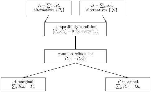
For compatible sharp observables, the products $R_{ab}=P_aQ_b$ are joint projectors. Summing over $b$ forgets the $B$ label and returns $P_a$; summing over $a$ forgets the $A$ label and returns $Q_b$.

Joint Born Probabilities

For a density operator $\rho$, the joint Born distribution is

$$p(a,b) = \operatorname{Tr}(\rho R_{ab}) = \operatorname{Tr}(\rho P_aQ_b).$$

For a pure state $\rho=|\psi\rangle\langle\psi|$,

$$p(a,b) = \langle\psi|P_aQ_b|\psi\rangle.$$

The marginals are exactly the individual Born probabilities:

$$\begin{aligned} \sum_b p(a,b) &=\operatorname{Tr}(\rho P_a), \\ \sum_a p(a,b) &=\operatorname{Tr}(\rho Q_b). \end{aligned}$$

Compatibility therefore permits a single state-independent joint measurement whose distribution has the correct marginals for every preparation. Merely writing down a joint distribution for two separate marginal distributions proves much less: one could always multiply those marginals, but that construction need not come from any fixed quantum measurement.

Operational Meaning for Ideal Sequential Measurements

Suppose Lüders measurements of $A$ and then $B$ yield outcomes $a,b$, with no intervening evolution. The joint probability is

$$p(a\text{ then }b) = \operatorname{Tr} \left( Q_bP_a\rho P_a \right).$$

Using cyclicity of the trace,

$$p(a\text{ then }b) = \operatorname{Tr} \left( \rho P_aQ_bP_a \right).$$

If $P_a$ and $Q_b$ commute, then

$$P_aQ_bP_a=P_aQ_b,$$

so

$$p(a\text{ then }b) = \operatorname{Tr}(\rho P_aQ_b).$$

Reversing the order gives the same result:

$$p(b\text{ then }a) = \operatorname{Tr}(\rho Q_bP_a) =p(a,b).$$

Conditioned on the joint outcome $(a,b)$, the ideal updated state is

$$\rho_{ab} = \frac{R_{ab}\rho R_{ab}} {\operatorname{Tr}(\rho R_{ab})},$$

provided $p(a,b)>0$. The detailed probability tree and state updates belong to Sequential Measurements.

This order independence concerns ideal projective instruments. An apparatus can append an extra outcome-dependent unitary or couple to unrecorded degrees of freedom while realizing the same projectors. Compatibility of observables does not make every such implementation mutually nondisturbing.

Degeneracy: Preserved Blocks, Not Arbitrary Bases

The slogan “commuting observables have the same eigenvectors” is imprecise in the presence of degeneracy. Commutation guarantees that a simultaneous basis can be chosen; it does not guarantee that every eigenbasis selected for one operator diagonalizes the other.

Consider

$$A= \begin{pmatrix} 1&0&0\\ 0&1&0\\ 0&0&2 \end{pmatrix}, \qquad B= \begin{pmatrix} 0&1&0\\ 1&0&0\\ 0&0&3 \end{pmatrix}.$$

The first two coordinate vectors are $A$ eigenvectors with eigenvalue $1$, but neither is a $B$ eigenvector. Because $A$ is proportional to the identity inside their two-dimensional subspace, $B$ may mix them without leaving that subspace. Directly,

$$[A,B]=0.$$

Diagonalizing $B$ inside the degenerate block gives

$$|+\rangle = \frac{|e_1\rangle+|e_2\rangle}{\sqrt2}, \qquad |-\rangle = \frac{|e_1\rangle-|e_2\rangle}{\sqrt2}.$$

The simultaneous labels are

$$\begin{array}{c|c|c} \text{state}&A\text{ eigenvalue}&B\text{ eigenvalue}\\ \hline |+\rangle&1&1\\ |-\rangle&1&-1\\ |e_3\rangle&2&3 \end{array}.$$

Here $B$ resolves the degeneracy of $A$. The detailed treatment of whether a family removes all residual degeneracy is Complete Sets of Commuting Observables. The corresponding ideal update within a degenerate eigenspace is treated in Degenerate Measurements and Lüders Rule.

Nondegenerate Observables

If $A$ has a nondegenerate spectrum and $[A,B]=0$, every one-dimensional $A$-eigenspace is preserved by $B$. Therefore

$$B|a_n\rangle=b_n|a_n\rangle.$$

In finite dimension one can define a function $f$ on the spectrum of $A$ by

$$f(a_n)=b_n.$$

Then

$$B=f(A).$$

Thus a compatible $B$ supplies no new refinement of a nondegenerate $A$ measurement: once $a_n$ is known, $b_n$ is determined. Compatibility and independence of labels are different questions.

Compatible Families

For a finite family of self-adjoint matrices

$$\left\lbrace A_1,\ldots,A_r \right\rbrace,$$

pairwise commutation,

$$[A_j,A_k]=0 \qquad \text{for all }j,k,$$

implies simultaneous diagonalizability. The proof proceeds recursively: diagonalize $A_1$, restrict $A_2$ to each preserved eigenspace, and continue inside the successively refined joint subspaces.

If $P^{(k)}_{a_k}$ is the spectral projector of $A_k$, the joint projectors are

$$R_{a_1\cdots a_r} = \prod_{k=1}^{r}P^{(k)}_{a_k}.$$

Pairwise commutation makes the product independent of ordering. A compatible family need not be complete: a nonzero $R_{a_1\cdots a_r}$ can still have rank greater than one.

Compatibility Is Not Completeness

Compatibility asks whether the alternatives can be jointly refined. Completeness asks whether the surviving joint alternatives are one-dimensional within a declared space or sector.

For example, on a Hilbert space with orbital angular momentum sectors,

$$[L^2,L_z]=0,$$

so $L^2$ and $L_z$ are compatible. Their labels $(\ell,m)$ may still leave other degrees of freedom, such as a radial quantum number, unspecified.

Likewise, the identity $I$ commutes with every observable but refines nothing. Compatibility is necessary for a CSCO, not sufficient.

Compatibility Is Not Statistical Independence

Joint measurability supplies a joint distribution, but it does not force that distribution to factorize:

$$p(a,b) \ne p_A(a)p_B(b)$$

in general.

For two qubits, consider

$$A=\sigma_z\otimes I, \qquad B=I\otimes\sigma_z.$$

The operators act on different tensor factors, so

$$[A,B]=0.$$

In the state

$$|\Phi^+\rangle = \frac{|00\rangle+|11\rangle}{\sqrt2},$$

the only joint outcomes are $(+1,+1)$ and $(-1,-1)$, each with probability $1/2$. Both marginals are unbiased, yet the outcomes are perfectly correlated:

$$\langle A\rangle=\langle B\rangle=0, \qquad \langle AB\rangle=1.$$

The probability structure of such examples is developed in Correlations and Covariance.

Compatibility Does Not Make Every State Sharp

Let $|a,b,\mu\rangle$ be a simultaneous eigenbasis. A general state can be a superposition

$$|\psi\rangle = \sum_{a,b,\mu} c_{ab\mu}|a,b,\mu\rangle.$$

Unless all nonzero coefficients share the same $a$ and $b$, the state has nonzero spread in one or both observables. Compatibility means that sharp joint alternatives exist and form a complete decomposition, not that the prepared state occupies only one of them.

A joint eigenstate can satisfy

$$\Delta A=\Delta B=0,$$

but a superposition of joint eigenstates can have

$$\Delta A>0, \qquad \Delta B>0.$$

Compatibility and Uncertainty

The Robertson relation reads

$$\Delta A\,\Delta B \ge \frac12 \left| \langle[A,B]\rangle \right|.$$

For compatible observables, the commutator lower bound vanishes:

$$[A,B]=0 \quad\Longrightarrow\quad \Delta A\,\Delta B\ge0.$$

This does not predict zero variances in an arbitrary state. It says that the commutator term supplies no positive lower bound here. The finite-dimensional common-eigenbasis theorem, rather than this inequality alone, establishes the existence of common sharp states. The covariance term in the stronger Robertson–Schrödinger relation may also be nonzero for a superposition of joint eigenstates. See General Uncertainty Relations for the derivation and equality conditions.

Standard Examples

Angular momentum

The total orbital angular momentum and one chosen component commute:

$$[L^2,L_z]=0.$$

The states $|\ell,m\rangle$ are simultaneous eigenstates:

$$L^2|\ell,m\rangle = \hbar^2\ell(\ell+1)|\ell,m\rangle,$$

and

$$L_z|\ell,m\rangle = \hbar m|\ell,m\rangle.$$

By contrast,

$$[L_x,L_z]=-i\hbar L_y\ne0,$$

so $L_x$ and $L_z$ are incompatible.

A symmetry and the Hamiltonian

If a parity-invariant Hamiltonian satisfies

$$[H,\Pi]=0,$$

its energy eigenspaces are preserved by parity. Energy eigenvectors can be chosen with definite parity. If an energy level is nondegenerate, its eigenvector is automatically a parity eigenvector; if it is degenerate, parity must be diagonalized inside that energy eigenspace.

For time-independent $H$ and parity, commutation of parity with the spectral measure of $H$ also makes its outcome probabilities conserved under the corresponding unitary evolution.

Spinless hydrogenic labels

For the ideal spinless Coulomb Hamiltonian,

$$[H,L^2]=[H,L_z]=[L^2,L_z]=0.$$

The labels $(n,\ell,m)$ can therefore be assigned simultaneously to bound states. The model-specific degeneracies and radial structure belong to the hydrogenic system pages; the label-completeness question belongs to the CSCO article.

Observables on separate tensor factors

Bounded operators of the form

$$A\otimes I \qquad\text{and}\qquad I\otimes B$$

always commute because

$$\begin{aligned} (A\otimes I)(I\otimes B) &=A\otimes B, \\ (I\otimes B)(A\otimes I) &=A\otimes B. \end{aligned}$$

This algebraic compatibility does not preclude correlations created by the state, as the two-qubit example above demonstrates.

Position and Momentum as a Contrast

Position and momentum obey the canonical relation

$$[x,p]=i\hbar I$$

on an appropriate common domain. Their spectral projective measurements do not possess a common sharp refinement. This incompatibility underlies the position–momentum uncertainty relation, though uncertainty, measurement disturbance, and noncommutativity should not be collapsed into one slogan.

The representation and domain qualifications for this equation are treated in Canonical Commutation Relations.

Infinite-Dimensional and Unbounded Operators

For bounded self-adjoint operators, the equation $AB=BA$ is defined on the whole Hilbert space and is equivalent to commutation of their spectral measures.

For unbounded self-adjoint operators, products such as $AB$ and $BA$ may have different domains. Verifying

$$AB|\psi\rangle=BA|\psi\rangle$$

on some dense common domain need not establish full measurement compatibility.

The robust condition is strong commutativity. If $E_A(\Delta)$ and $E_B(\Gamma)$ are the spectral projections associated with Borel sets $\Delta$ and $\Gamma$, require

$$E_A(\Delta)E_B(\Gamma) = E_B(\Gamma)E_A(\Delta)$$

for every pair of Borel sets. Then

$$E(\Delta\times\Gamma) = E_A(\Delta)E_B(\Gamma)$$

defines a joint projection-valued measure. This is the infinite-dimensional counterpart of $R_{ab}=P_aQ_b$.

Domain statements should therefore specify what commutes, on which domain, and whether spectral projections commute. A formal vanishing commutator does not establish this spectral condition.

Generalized Measurements: A Different Criterion

For POVMs $\{E_a\}$ and $\{F_b\}$, joint measurability means that there is a POVM $\{G_{ab}\}$ such that

$$\sum_bG_{ab}=E_a, \qquad \sum_aG_{ab}=F_b.$$

If all effects $E_a$ commute with all effects $F_b$, then

$$G_{ab}=E_aF_b$$

is a joint POVM, so commutation is sufficient. Unlike the sharp projective case, it is not necessary: sufficiently unsharp noncommuting measurements can be jointly measurable.

Thus the equivalence

$$\text{compatibility} \quad\Longleftrightarrow\quad \text{commutation}$$

belongs specifically to sharp projective observables. See POVMs: First Encounter for the generalized framework.

Common Pitfalls

One common vector is insufficient. Compatibility concerns a complete joint decomposition of the declared space. Two observables may share a sharp state while remaining incompatible on its orthogonal complement.

Joint probabilities can be correlated. Commutation allows a joint measurement; the state determines whether its outcomes factorize. Entangled states and classical mixtures can both produce correlations between compatible observables.

Outcome statistics do not fix disturbance. Commuting projectors give order-independent Lüders statistics. A device that adds an extra transformation can disturb another compatible observable, as Exercise 4 illustrates.

Unsharp measurements use a different criterion. Noncommuting POVM effects can have a common parent measurement. Constructing its positive effects and checking both marginals is the direct test.

Exercises

Exercise 1: Common basis implies commutation

Suppose finite-dimensional $A$ and $B$ have an orthonormal simultaneous eigenbasis $|n\rangle$:

$$A|n\rangle=a_n|n\rangle, \qquad B|n\rangle=b_n|n\rangle.$$

Prove that $[A,B]=0$.

Solution

On every basis vector,

$$\begin{aligned} AB|n\rangle &=a_nb_n|n\rangle, \\ BA|n\rangle &=b_na_n|n\rangle. \end{aligned}$$

Therefore $[A,B]|n\rangle=0$ for every $n$. Because the vectors $|n\rangle$ span the Hilbert space and the commutator is linear,

$$[A,B]|\psi\rangle=0$$

for every $|\psi\rangle$. Hence $[A,B]=0$.

Exercise 2: Resolve a degenerate block

For

$$A= \begin{pmatrix} 1&0&0\\ 0&1&0\\ 0&0&2 \end{pmatrix}, \qquad B= \begin{pmatrix} 0&1&0\\ 1&0&0\\ 0&0&3 \end{pmatrix},$$

verify that $A$ and $B$ commute and find an orthonormal simultaneous eigenbasis.

Solution

Both matrices preserve

$$\operatorname{span} \left\lbrace |e_1\rangle,|e_2\rangle \right\rbrace$$

and $\operatorname{span}\{|e_3\rangle\}$. On the first block, $A$ is the identity times $1$, so it commutes with the restriction of $B$. On the second block both are scalar. Hence $[A,B]=0$.

The eigenvectors of the first block of $B$ are

$$\begin{aligned} |+\rangle &= \frac{|e_1\rangle+|e_2\rangle}{\sqrt2}, \\ |-\rangle &= \frac{|e_1\rangle-|e_2\rangle}{\sqrt2}. \end{aligned}$$

Together with $|e_3\rangle$, they form an orthonormal simultaneous eigenbasis. Their joint eigenvalue pairs are

$$(1,1), \qquad (1,-1), \qquad (2,3).$$

Exercise 3: Joint projectors

Let $\{P_a\}$ and $\{Q_b\}$ be commuting PVMs. Show that

$$R_{ab}=P_aQ_b$$

is a PVM and has $P_a$ and $Q_b$ as marginals.

Solution

Because $P_a$ and $Q_b$ commute,

$$R_{ab}^{\dagger} =Q_bP_a =P_aQ_b =R_{ab}$$

and

$$R_{ab}^2 =P_a^2Q_b^2 =R_{ab}.$$

For distinct joint outcomes,

$$R_{ab}R_{a'b'} = \delta_{aa'}\delta_{bb'}R_{ab}.$$

Finally,

$$\sum_{a,b}R_{ab} = \left(\sum_aP_a\right) \left(\sum_bQ_b\right) =I,$$

and

$$\sum_bR_{ab}=P_a, \qquad \sum_aR_{ab}=Q_b.$$

Thus the $R_{ab}$ form a projective measurement with the required marginals.

Exercise 4: A compatible observable can still be disturbed

On two qubits let $A=\sigma_z\otimes I$ and $B=I\otimes\sigma_z$. An apparatus measures $A$ projectively and then applies $I\otimes\sigma_x$, regardless of the result. Does it still give the correct $A$ probabilities? Starting from $|00\rangle$, compare a later measurement of $B$ with measuring $B$ before using the apparatus.

Solution

Its outcome operators are $M_a=(I\otimes\sigma_x)P_a$, so $M_a^\dagger M_a=P_a$. Thus it realizes the same sharp $A$ statistics, and $[A,B]=0$ still holds.

Initially $B$ gives $+1$ with certainty. The apparatus records $A=+1$ and leaves $|01\rangle$, so the subsequent $B$ measurement gives $-1$ with certainty. The extra flip even preserves the recorded $A$ eigenspace, but it disturbs $B$. Compatibility guarantees an appropriate joint or nondisturbing implementation; it does not constrain every device with those effects.

Exercise 5: Order-independent ideal statistics

Let $P_aQ_b=Q_bP_a$. Starting from the Lüders sequential probabilities, show that measuring $A$ then $B$ or $B$ then $A$ gives the same joint distribution.

Solution

For $A$ then $B$,

$$\begin{aligned} p(a\text{ then }b) &=\operatorname{Tr}(Q_bP_a\rho P_a) \\ &=\operatorname{Tr}(\rho P_aQ_bP_a) \\ &=\operatorname{Tr}(\rho P_aQ_b). \end{aligned}$$

For the reverse order,

$$\begin{aligned} p(b\text{ then }a) &=\operatorname{Tr}(P_aQ_b\rho Q_b) \\ &=\operatorname{Tr}(\rho Q_bP_aQ_b) \\ &=\operatorname{Tr}(\rho Q_bP_a). \end{aligned}$$

Since $P_aQ_b=Q_bP_a$, both expressions equal

$$\operatorname{Tr}(\rho R_{ab}).$$

Exercise 6: Compatible but correlated

For

$$A=\sigma_z\otimes I, \qquad B=I\otimes\sigma_z,$$

and

$$|\Phi^+\rangle = \frac{|00\rangle+|11\rangle}{\sqrt2},$$

compute the joint distribution and covariance.

Solution

The state has amplitude only on $|00\rangle$ and $|11\rangle$. Therefore

$$p(+1,+1)=\frac12, \qquad p(-1,-1)=\frac12,$$

with the two mixed-sign probabilities equal to zero. Hence

$$\langle A\rangle=0, \qquad \langle B\rangle=0,$$

while

$$\langle AB\rangle=1.$$

The covariance is

$$\operatorname{Cov}(A,B) = \langle AB\rangle - \langle A\rangle\langle B\rangle =1.$$

The observables are compatible because they commute, but their outcomes are not independent in this state.

Exercise 7: Nondegeneracy and functional dependence

Let $A$ be a self-adjoint matrix with nondegenerate eigenvalues $a_n$, let $B$ also be self-adjoint, and suppose $[A,B]=0$. Show that $B=f(A)$ for some function $f$ defined on the spectrum of $A$.

Solution

Each eigenspace of $A$ is one-dimensional. Since $B$ preserves every $A$-eigenspace,

$$B|a_n\rangle=b_n|a_n\rangle$$

for some real $b_n$. Define $f(a_n)=b_n$. Spectral calculus gives

$$\begin{aligned} f(A) &= \sum_n f(a_n)|a_n\rangle\langle a_n|, \\ &= \sum_n b_n|a_n\rangle\langle a_n| \\ &=B. \end{aligned}$$

Because the spectrum is finite, a polynomial interpolating the values $b_n$ at the points $a_n$ may be used for $f$.

Exercise 8: Jointly measurable unsharp spin components

For $a,b\in\{+1,-1\}$, define qubit effects

$$G_{ab} = \frac14 \left[ I+\eta(a\sigma_x+b\sigma_z) \right].$$

Show that $\{G_{ab}\}$ is a joint POVM for unsharp $x$ and $z$ spin measurements when $0\le\eta\le1/\sqrt2$, even though the marginal effects do not commute when $\eta>0$.

Solution

The Pauli coefficient vector inside the bracket has length $\eta\sqrt2$. Its eigenvalues are

$$\lambda_{\pm} = \frac14 \left(1\pm\eta\sqrt2\right).$$

Thus every $G_{ab}$ is positive exactly when

$$0\le\eta\le\frac1{\sqrt2}.$$

Summing over $b$ gives

$$\sum_bG_{ab} = \frac12(I+a\eta\sigma_x) \equiv E_a^{(x)},$$

and summing over $a$ gives

$$\sum_aG_{ab} = \frac12(I+b\eta\sigma_z) \equiv E_b^{(z)}.$$

Also $\sum_{a,b}G_{ab}=I$, so the $G_{ab}$ form a parent POVM for both marginals. For $\eta>0$,

$$[E_a^{(x)},E_b^{(z)}] = \frac{ab\eta^2}{4} [\sigma_x,\sigma_z] \ne0.$$

This example shows why joint measurability and effect commutation are not equivalent for unsharp POVMs.

References

• P. Busch, P. J. Lahti, J.-P. Pellonpää, and K. Ylinen, Quantum Measurement, Springer, 2016. Publisher.
• B. C. Hall, Quantum Theory for Mathematicians, Springer, 2013. Publisher.
• J. J. Sakurai and J. Napolitano, Modern Quantum Mechanics, 3rd ed., Cambridge University Press, 2020, Chapter 1. Publisher.