Weak Values

A weak value is a conditional response coefficient obtained from a weak measurement followed by postselection. For a preselected pure state $\lvert\psi_i\rangle$, a later postselected pure state $\lvert\psi_f\rangle$, and an observable $A$, the standard weak value is

$$A_w = \frac{ \langle\psi_f|A|\psi_i\rangle }{ \langle\psi_f|\psi_i\rangle }, \qquad \langle\psi_f|\psi_i\rangle\ne0.$$

This expression is simple enough to invite overinterpretation. Operationally, $A_w$ is not a single-shot detector reading and not usually an eigenvalue. It is the complex coefficient that controls the first-order response of a weak pointer in the subensemble that passes the final selection.

The useful slogan is:

$$\text{weak value} \quad=\quad \text{transition-amplitude ratio} \quad=\quad \text{postselected weak-response coefficient}.$$

Helpful background. Weak measurements explains small coupling and accumulated backaction. The derivation below uses the von Neumann pointer model.

Weak responses in a postselected ensemble

A weak-value experiment has three ingredients:

1. prepare an initial ensemble in $\lvert\psi_i\rangle$;
2. weakly couple the system to a meter with a coupling weak enough for the chosen postselection;
3. perform a later measurement and keep only runs with outcome $\lvert\psi_f\rangle$.

The retained data set is not the original ensemble. It is a postselected subensemble with zeroth-order success probability

$$p_f^{(0)} = \lvert\langle\psi_f|\psi_i\rangle\rvert^2.$$

When this probability is small, the denominator of $A_w$ is small and the weak value can become large. The same small denominator also means that the successful sample is rare and sensitive to higher-order effects, technical background, and statistical uncertainty.

Pointer Model

Use the standard von Neumann meter. The system observable $A$ couples impulsively to a pointer coordinate $Q$ through its conjugate momentum $P$:

$$U_g = \exp \!\left( -\frac{i}{\hbar}g A\otimes P \right), \qquad [Q,P]=i\hbar.$$

Let the initial pointer state be $\lvert\phi\rangle$, centered so that $\langle Q\rangle_\phi=\langle P\rangle_\phi=0$. After the coupling and successful postselection, the unnormalized pointer state is

$$\lvert\Phi_f\rangle = \langle\psi_f|U_g|\psi_i\rangle \lvert\phi\rangle.$$

For weak coupling,

$$\langle\psi_f|U_g|\psi_i\rangle = \langle\psi_f|\psi_i\rangle \left[ 1 - \frac{i g}{\hbar} A_w P + O(g^2) \right].$$

More explicitly, the second-order term contains the weak value of $A^2$:

$$\langle\psi_f|U_g|\psi_i\rangle = \langle\psi_f|\psi_i\rangle \left[ 1 - \frac{i g}{\hbar}A_w P - \frac{g^2}{2\hbar^2}(A^2)_w P^2 + O(g^3) \right],$$

where

$$(A^2)_w = \frac{ \langle\psi_f|A^2|\psi_i\rangle }{ \langle\psi_f|\psi_i\rangle }.$$

These are expansions acting on a pointer with the needed finite momentum moments; they are not operator-norm expansions in the unbounded operator $P$. The ratios after postselection must be controlled. For example, $|g A_w|\Delta P/\hbar\ll1$ keeps the first-order correction small, while $g^2|(A^2)_w|\sqrt{\langle P^4\rangle}/\hbar^2\ll1$ controls the next term. Still higher terms must also remain negligible.

Pointer Shifts

For a real centered Gaussian pointer with no initial $Q$-$P$ correlation, the first-order shifts are

$$\Delta\langle Q\rangle_f = g\,\operatorname{Re} A_w,$$

and

$$\Delta\langle P\rangle_f = \frac{2g(\Delta P)^2}{\hbar} \operatorname{Im} A_w.$$

The real part shifts the pointer position. The imaginary part changes the conjugate momentum distribution. For this centered pointer, however, the total postselection probability has no linear change, since that term is $2g\operatorname{Im}(A_w)\langle P\rangle/\hbar=0$. A nonzero initial position–momentum covariance adds $2g\operatorname{Im}(A_w)\operatorname{Cov}(Q,P)/\hbar$ to the position shift (Jozsa, 2007).

The normalized postselected pointer mean is a conditional statistic:

$$\langle Q\rangle_f = \frac{ \langle\Phi_f|Q|\Phi_f\rangle }{ \langle\Phi_f|\Phi_f\rangle }.$$

It is measured by averaging many successful trials. A single retained event does not display the weak value.

Spectral Form

If

$$A=\sum_a a\,\Pi_a,$$

then

$$A_w = \sum_a a\,(\Pi_a)_w, \qquad (\Pi_a)_w = \frac{ \langle\psi_f|\Pi_a|\psi_i\rangle }{ \langle\psi_f|\psi_i\rangle }.$$

The quantities $(\Pi_a)_w$ sum to one:

$$\sum_a(\Pi_a)_w=1.$$

They are not ordinary probabilities. They can be negative or complex, and they need not lie between $0$ and $1$. This is one way to see how $A_w$ can lie outside the eigenvalue range of $A$: the weak value is a weighted transition-amplitude ratio, not a convex average with positive weights.

An imaginary weak value

Take $A=\sigma_z$, $|\psi_i\rangle=|+x\rangle$, and $|\psi_f\rangle=|+y\rangle=(|0\rangle+i|1\rangle)/\sqrt2$. Then

$$A_w=\frac{1+i}{1-i}=i, \qquad p_f^{(0)}=\frac12.$$

The centered Gaussian pointer has no first-order position displacement, but its momentum shifts by $2g(\Delta P)^2/\hbar$. Measuring only position would miss this response. A Hermitian observable still has real projective outcomes: the complex ratio describes two aspects of a conditional pointer distribution.

Ordinary Limits

Weak values reduce to familiar quantities in special cases.

If the preselected and postselected states are the same,

$$\lvert\psi_f\rangle=\lvert\psi_i\rangle,$$

then

$$A_w = \langle\psi_i|A|\psi_i\rangle.$$

If the postselected state is an eigenstate of $A$,

$$A\lvert a\rangle=a\lvert a\rangle, \qquad \langle a|\psi_i\rangle\ne0,$$

and $\lvert\psi_f\rangle=\lvert a\rangle$, then

$$A_w=a.$$

Anomalous weak values therefore require a nontrivial relation among preparation, observable, and postselection. They are not produced merely by making a meter noisy.

A Qubit Example

Let

$$\lvert\psi_i\rangle = \lvert +x\rangle = \frac{ \lvert +z\rangle+\lvert -z\rangle }{\sqrt 2},$$

and choose the postselected state

$$\lvert\psi_f\rangle = \frac{ \lvert +z\rangle-\alpha\lvert -z\rangle }{ \sqrt{1+\alpha^2} }, \qquad 0\le\alpha\lt1.$$

For $A=\sigma_z$,

$$\langle\psi_f|\psi_i\rangle = \frac{1-\alpha} {\sqrt{2(1+\alpha^2)}},$$

while

$$\langle\psi_f|\sigma_z|\psi_i\rangle = \frac{1+\alpha} {\sqrt{2(1+\alpha^2)}}.$$

Thus

$$(\sigma_z)_w = \frac{1+\alpha}{1-\alpha}.$$

For $\alpha$ close to $1$, this weak value is much larger than the eigenvalue range $[-1,1]$. The same limit makes the postselection probability small:

$$p_f^{(0)} = \frac{(1-\alpha)^2} {2(1+\alpha^2)}.$$

The anomalous value and rare postselection arise from the same small overlap. An exact finite-coupling calculation shows why the first-order prediction cannot diverge in a fixed apparatus.

For a real Gaussian $\phi(q)\propto e^{-q^2/(4\sigma^2)}$, the successful pointer amplitude is

$$\Phi_f(q)=\frac{\phi(q-g)-\alpha\phi(q+g)}{\sqrt{2(1+\alpha^2)}}.$$

The two packets overlap by $S=e^{-g^2/(2\sigma^2)}$. Their cross term has zero first moment about the origin, giving

$$p_f=\frac{1+\alpha^2-2\alpha S}{2(1+\alpha^2)}, \qquad \langle Q\rangle_f= \frac{g(1-\alpha^2)}{1+\alpha^2-2\alpha S}.$$

For $\alpha=0.8$, the formal weak value is $9$. At $g=0.02\sigma$, the exact mean is about $0.1786\sigma$, close to $gA_w=0.18\sigma$. At $g=0.2\sigma$, it is about $1.004\sigma$, far from $1.8\sigma$. At any fixed nonzero $g$, taking $\alpha\to1$ gives zero mean, not an infinite displacement. In that limit the successful distribution has an antisymmetric amplitude and the zero-coupling success probability vanishes; the limits do not commute.

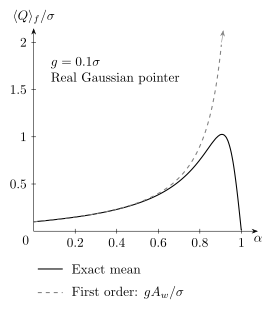
For fixed $g=0.1\sigma$, the exact Gaussian-pointer mean bends away from $gA_w$ when the postselection is too nearly orthogonal. Small apparatus coupling alone does not ensure a valid expansion for a rare selected ensemble.

Time-Dependent Form

If the weak coupling occurs at an intermediate time $t$ between preparation at $t_i$ and postselection at $t_f$, unitary evolution gives

$$A_w(t) = \frac{ \langle\psi_f| U(t_f,t)\,A\,U(t,t_i) |\psi_i\rangle }{ \langle\psi_f| U(t_f,t_i) |\psi_i\rangle }.$$

This formula is often useful, but the notation should not be read as assigning an ordinary possessed value to the system at time $t$. It is a conditional amplitude ratio for a particular preparation, dynamics, weak coupling, and final filter.

Mixed States and Effects

For a mixed initial state $\rho_i$ and a final postselection represented by an effect $E_f$, the common trace form is

$$A_w = \frac{ \operatorname{Tr}(E_f A\rho_i) }{ \operatorname{Tr}(E_f\rho_i) }, \qquad \operatorname{Tr}(E_f\rho_i)\ne0.$$

This expression keeps the time ordering appropriate to a weak measurement of $A$ before the final effect $E_f$. Any evolution after the weak interaction is incorporated by propagating the final effect backward with its adjoint map. If the weak interaction itself includes other first-order disturbance, the standard formula need not describe the response. When the final system is simply discarded, the final effect is sufficient for the pointer statistics; its subsequent state update is irrelevant. The numerator is not just a classical conditional expectation.

Statistical Estimation

In an experiment, one estimates weak values from many trials. Let $N$ be the number of prepared systems and let $N_f$ be the number that pass postselection. Roughly,

$$N_f\approx N p_f,$$

where $p_f$ includes the effects of the weak measurement and technical imperfections. The uncertainty of the pointer mean scales with the number of successful runs, not with the number initially prepared:

$$\delta\langle Q\rangle_f \sim \frac{\sigma_{Q,f}}{\sqrt{N_f}}.$$

Here $\sigma_{Q,f}$ is the standard deviation in the selected output distribution, which need not equal the initial pointer width. Independent finite-variance successful samples are assumed.

A large $\operatorname{Re}A_w$ can amplify a pointer displacement in the retained ensemble, but it can simultaneously reduce $N_f$. Whether this improves a real measurement depends on the noise model: technical offsets, detector saturation, background counts, and imperfect postselection matter. Weak-value amplification is therefore a metrological technique with conditions, not a general way to beat quantum statistics.

Interpretive Caution

Weak values have been important in discussions of measurement, contextuality, quantum paradoxes, and pre/postselected ensembles. Those discussions can be illuminating, but they should be separated from the basic measurement theory.

The settled technical statement is that weak values are experimentally accessible response coefficients under specified weak-coupling and postselection conditions. Stronger claims about what a quantum system “really had” between two measurements require an interpretation and should not be presented as automatic consequences of the formula.

For broader foundations context, see What These Experiments Do and Do Not Prove.

Exercises

Same preselection and postselection

Show that if $\lvert\psi_f\rangle=\lvert\psi_i\rangle$, the weak value of $A$ is the ordinary expectation value of $A$ in the state $\lvert\psi_i\rangle$.

Solution

Substitute $\lvert\psi_f\rangle=\lvert\psi_i\rangle$:

$$A_w = \frac{ \langle\psi_i|A|\psi_i\rangle }{ \langle\psi_i|\psi_i\rangle }.$$

For a normalized state, $\langle\psi_i|\psi_i\rangle=1$, so

$$A_w=\langle\psi_i|A|\psi_i\rangle.$$

Eigenstate postselection

Let $A\lvert a\rangle=a\lvert a\rangle$ and let $\lvert\psi_f\rangle=\lvert a\rangle$. Assume $\langle a|\psi_i\rangle\ne0$. Show that $A_w=a$.

Solution

Using $\langle a|A=a\langle a|$ for Hermitian $A$,

$$A_w = \frac{ \langle a|A|\psi_i\rangle }{ \langle a|\psi_i\rangle } = \frac{ a\langle a|\psi_i\rangle }{ \langle a|\psi_i\rangle } = a.$$

Largest displacement at fixed coupling

Keep the real Gaussian pointer and qubit preparation in the example above, with fixed $g>0$ and $\sigma>0$. Vary only $0\le\alpha\le1$. Find the postselection that maximizes the exact mean $\langle Q\rangle_f$, its success probability, and the selected position variance. What happens as $g/\sigma\to0$ along this optimum?

Solution

Write $S=e^{-g^2/(2\sigma^2)}$, so $0<S<1$. Differentiating the exact mean gives

$$\frac{d\langle Q\rangle_f}{d\alpha} =\frac{2g[S(1+\alpha^2)-2\alpha]}{(1+\alpha^2-2\alpha S)^2}.$$

The derivative changes from positive to negative at

$$\alpha_* = \frac{S}{1+\sqrt{1-S^2}}, \qquad \max_{0\le\alpha\le1}\langle Q\rangle_f =\frac{g}{\sqrt{1-S^2}}, \qquad p_f(\alpha_*)=\frac{1-S^2}{2}.$$

To check the width, the translated packets have second moment $\sigma^2+g^2$, while $\int q^2\phi(q-g)\phi(q+g)\,dq=\sigma^2S$. Hence

$$\langle Q^2\rangle_f =\sigma^2+\frac{g^2(1+\alpha^2)}{1+\alpha^2-2\alpha S}.$$

At the optimum, $2\alpha_*/(1+\alpha_*^2)=S$. Subtracting the squared mean then gives $\operatorname{Var}_f Q=\sigma^2$ exactly; this equality does not make the selected distribution Gaussian.

As $g/\sigma\to0$, the maximum mean approaches $\sigma$, while $p_f(\alpha_*)\sim g^2/(2\sigma^2)$ vanishes. For $N$ independent preparations, estimating that mean from the selected trials requires $Np_f\gg1$, with standard error approximately $\sigma/\sqrt{Np_f}$. The finite mean in this joint limit describes an increasingly rare ensemble. It is neither a displacement at exactly zero coupling nor a universal bound for other pointer states or preparations.

Pointer shift from the first-order state

Assume a centered real Gaussian pointer with no initial $Q$-$P$ correlation. Starting from

$$\lvert\Phi_f\rangle \propto \left( 1 - \frac{i g}{\hbar}A_w P \right) \lvert\phi\rangle,$$

show that the first-order position shift is $g\,\operatorname{Re}A_w$.

Solution

Write $A_w=a+ib$. To first order in $g$,

$$\langle Q\rangle_f = \langle Q\rangle_\phi + \frac{i g}{\hbar} \left( A_w^*\langle P Q\rangle_\phi - A_w\langle QP\rangle_\phi \right).$$

For a centered real Gaussian with no $Q$-$P$ correlation,

$$\langle Q\rangle_\phi=0, \qquad \langle QP\rangle_\phi=\frac{i\hbar}{2}, \qquad \langle P Q\rangle_\phi=-\frac{i\hbar}{2}.$$

Substitution gives

$$\langle Q\rangle_f = g a = g\,\operatorname{Re}A_w.$$

References

• Y. Aharonov, D. Z. Albert, and L. Vaidman, “How the result of a measurement of a component of the spin of a spin-1/2 particle can turn out to be 100,” Physical Review Letters 60, 1351–1354 (1988). Article.
• J. Dressel, M. Malik, F. M. Miatto, A. N. Jordan, and R. W. Boyd, “Colloquium: Understanding quantum weak values: Basics and applications,” Reviews of Modern Physics 86, 307–316 (2014). Article.
• I. M. Duck, P. M. Stevenson, and E. C. G. Sudarshan, “The sense in which a ‘weak measurement’ of a spin-1/2 particle’s spin component yields a value 100,” Physical Review D 40, 2112–2117 (1989). Article.
• R. Jozsa, “Complex weak values in quantum measurement,” Physical Review A 76, 044103 (2007). Article.